RADAR 2A product#
In this tutorial, we will provide the foundations to use GPM-API to download, manipulate and analyze data from the Global Precipitation Measurement (GPM) 2A radar products.
Please note that GPM-API also enable access and analysis tools for the entire GPM constellation of passive microwave sensors as well as the IMERG precipitation products. For detailed information and additional tutorials, please refer to the others GPM-API tutorials.
First, let’s import the package required in this tutorial.
[ ]:
import datetime

import cartopy.crs as ccrs
import matplotlib.pyplot as plt
import numpy as np
import xarray as xr
import ximage  # noqa

import gpm
from gpm.utils.geospatial import (
    get_circle_coordinates_around_point,
    get_country_extent,
    get_geographic_extent_around_point,
)
Using the available_products function, users can obtain a list of all GPM products that can be downloaded and opened into CF-compliant xarray datasets.
[ ]:
gpm.available_products(product_types="RS") # research products
['1A-GMI',
 '1A-TMI',
 '1B-GMI',
 '1B-Ka',
 '1B-Ku',
 '1B-PR',
 '1B-TMI',
 '1C-AMSR2-GCOMW1',
 '1C-AMSRE-AQUA',
 '1C-AMSUB-NOAA15',
 '1C-AMSUB-NOAA16',
 '1C-AMSUB-NOAA17',
 '1C-ATMS-NOAA20',
 '1C-ATMS-NOAA21',
 '1C-ATMS-NPP',
 '1C-GMI',
 '1C-GMI-R',
 '1C-MHS-METOPA',
 '1C-MHS-METOPB',
 '1C-MHS-METOPC',
 '1C-MHS-NOAA18',
 '1C-MHS-NOAA19',
 '1C-SAPHIR-MT1',
 '1C-SSMI-F08',
 '1C-SSMI-F10',
 '1C-SSMI-F11',
 '1C-SSMI-F13',
 '1C-SSMI-F14',
 '1C-SSMI-F15',
 '1C-SSMIS-F16',
 '1C-SSMIS-F17',
 '1C-SSMIS-F18',
 '1C-SSMIS-F19',
 '1C-TMI',
 '2A-AMSR2-GCOMW1',
 '2A-AMSR2-GCOMW1-CLIM',
 '2A-AMSRE-AQUA-CLIM',
 '2A-AMSUB-NOAA15-CLIM',
 '2A-AMSUB-NOAA16-CLIM',
 '2A-AMSUB-NOAA17-CLIM',
 '2A-ATMS-NOAA20',
 '2A-ATMS-NOAA20-CLIM',
 '2A-ATMS-NOAA21',
 '2A-ATMS-NOAA21-CLIM',
 '2A-ATMS-NPP',
 '2A-ATMS-NPP-CLIM',
 '2A-DPR',
 '2A-ENV-DPR',
 '2A-ENV-Ka',
 '2A-ENV-Ku',
 '2A-ENV-PR',
 '2A-GMI',
 '2A-GMI-CLIM',
 '2A-GPM-SLH',
 '2A-Ka',
 '2A-Ku',
 '2A-MHS-METOPA',
 '2A-MHS-METOPA-CLIM',
 '2A-MHS-METOPB',
 '2A-MHS-METOPB-CLIM',
 '2A-MHS-METOPC',
 '2A-MHS-METOPC-CLIM',
 '2A-MHS-NOAA18',
 '2A-MHS-NOAA18-CLIM',
 '2A-MHS-NOAA19',
 '2A-MHS-NOAA19-CLIM',
 '2A-PR',
 '2A-SAPHIR-MT1',
 '2A-SAPHIR-MT1-CLIM',
 '2A-SSMI-F08-CLIM',
 '2A-SSMI-F10-CLIM',
 '2A-SSMI-F11-CLIM',
 '2A-SSMI-F13-CLIM',
 '2A-SSMI-F14-CLIM',
 '2A-SSMI-F15-CLIM',
 '2A-SSMIS-F16',
 '2A-SSMIS-F16-CLIM',
 '2A-SSMIS-F17',
 '2A-SSMIS-F17-CLIM',
 '2A-SSMIS-F18',
 '2A-SSMIS-F18-CLIM',
 '2A-SSMIS-F19',
 '2A-SSMIS-F19-CLIM',
 '2A-TMI-CLIM',
 '2A-TRMM-SLH',
 '2B-GPM-CORRA',
 '2B-GPM-CSAT',
 '2B-GPM-CSH',
 '2B-TRMM-CORRA',
 '2B-TRMM-CSAT',
 '2B-TRMM-CSH',
 'IMERG-FR']
Let’s have a look at the available 2A RADAR products:
[ ]:
gpm.available_products(product_categories="RADAR", product_levels="2A")
['2A-DPR',
 '2A-ENV-DPR',
 '2A-ENV-Ka',
 '2A-ENV-Ku',
 '2A-ENV-PR',
 '2A-GPM-SLH',
 '2A-Ka',
 '2A-Ku',
 '2A-PR',
 '2A-TRMM-SLH']
In this tutorial, we will use the 2A-DPR product which provides the GPM Dual-frequency Precipitation Radar (DPR) reflectivities and associated precipitation retrievals.
1. Download Data#
Now let’s download the 2A-DPR product over a couple of hours.
To download GPM data with GPM-API, you have to previously create a NASA Earthdata and/or NASA PPS account. We provide a step-by-step guide on how to set up your accounts in the official GPM-API documentation.
[ ]:
# Specify the time period you are interested in
start_time = datetime.datetime.strptime("2023-08-20 20:00:00", "%Y-%m-%d %H:%M:%S")
end_time = datetime.datetime.strptime("2023-08-21 00:00:00", "%Y-%m-%d %H:%M:%S")
# Specify the product and product type
product = "2A-DPR"  # 2A-PR
product_type = "RS"
storage = "GES_DISC"
# Specify the version
version = 7
[ ]:
# Download the data
gpm.download(
    product=product,
    product_type=product_type,
    version=version,
    start_time=start_time,
    end_time=end_time,
    storage=storage,
    force_download=False,
    verbose=True,
    progress_bar=True,
    check_integrity=False,
)
All the available GPM 2A-DPR product files are already on disk.
Once, the data are downloaded on disk, let’s load the 2A-DPR product and look at the dataset structure.
2. Load Data#
With GPM-API, the name granule is used to refer to a single file, while the name dataset is used to refer to a collection of granules.
GPM-API enables to open single or multiple granules into xarray, a software designed for working with labeled multi-dimensional arrays.
The
gpm.open_granule_dataset(filepath)opens a singlescan_modeof a granule into axarray.Datasetobject by providing the path of the file of interest.The
gpm.open_granule_datatree(filepath)opens allscan_modesof granule into axarray.DataTreeobject by providing the path of the file of interest.The
gpm.open_datasetandgpm.open_datatreefunctions enable to open a collection of granules over a period of interest intoxarray.Datasetandxarray.DataTreeobjects respectively.
[ ]:
# Load the 2A-DPR dataset
ds = gpm.open_dataset(
    product=product,
    product_type=product_type,
    version=version,
    start_time=start_time,
    end_time=end_time,
)
ds
'scan_mode' has not been specified. Default to FS.
<xarray.Dataset> Size: 14GB
Dimensions:                       (cross_track: 49, along_track: 20573,
                                   nfreqHI: 3, range: 176, nNode: 5,
                                   nbinSZP: 7, radar_frequency: 2, nNUBF: 3,
                                   method: 6, three: 3, foreBack: 2,
                                   nearFar: 2, nsdew: 3, four: 4, nNP: 4,
                                   XYZ: 3, DSD_params: 2)
Coordinates: (12/16)
    sunLocalTime                  (cross_track, along_track) float32 4MB dask.array<chunksize=(49, 614), meta=np.ndarray>
    height                        (cross_track, along_track, range) float32 710MB dask.array<chunksize=(49, 614, 176), meta=np.ndarray>
    dataQuality                   (along_track, radar_frequency) float32 165kB dask.array<chunksize=(614, 2), meta=np.ndarray>
    SCorientation                 (along_track) float32 82kB dask.array<chunksize=(614,), meta=np.ndarray>
    lon                           (cross_track, along_track) float32 4MB 117....
    lat                           (cross_track, along_track) float32 4MB -52....
    ...                            ...
    gpm_along_track_id            (along_track) int64 165kB ...
  * range                         (range) int64 1kB 1 2 3 4 ... 173 174 175 176
    gpm_range_id                  (range) int64 1kB ...
  * radar_frequency               (radar_frequency) <U2 16B 'Ku' 'Ka'
  * DSD_params                    (DSD_params) <U2 16B 'Nw' 'Dm'
    crsWGS84                      int64 8B 0
Dimensions without coordinates: cross_track, along_track, nfreqHI, nNode,
                                nbinSZP, nNUBF, method, three, foreBack,
                                nearFar, nsdew, four, nNP, XYZ
Data variables: (12/139)
    flagBB                        (cross_track, along_track) float64 8MB dask.array<chunksize=(49, 614), meta=np.ndarray>
    binBBPeak                     (cross_track, along_track) float32 4MB dask.array<chunksize=(49, 614), meta=np.ndarray>
    binBBTop                      (cross_track, along_track) float32 4MB dask.array<chunksize=(49, 614), meta=np.ndarray>
    binDFRmMLBottom               (cross_track, along_track) float32 4MB dask.array<chunksize=(49, 614), meta=np.ndarray>
    binDFRmMLTop                  (cross_track, along_track) float32 4MB dask.array<chunksize=(49, 614), meta=np.ndarray>
    binBBBottom                   (cross_track, along_track) float32 4MB dask.array<chunksize=(49, 614), meta=np.ndarray>
    ...                            ...
    precipWaterIntegrated_Liquid  (cross_track, along_track) float32 4MB dask.array<chunksize=(49, 614), meta=np.ndarray>
    precipWaterIntegrated_Solid   (cross_track, along_track) float32 4MB dask.array<chunksize=(49, 614), meta=np.ndarray>
    precipWaterIntegrated         (cross_track, along_track) float32 4MB dask.array<chunksize=(49, 614), meta=np.ndarray>
    dBNw                          (cross_track, along_track, range) float32 710MB dask.array<chunksize=(49, 614, 176), meta=np.ndarray>
    Dm                            (cross_track, along_track, range) float32 710MB dask.array<chunksize=(49, 614, 176), meta=np.ndarray>
    Nw                            (cross_track, along_track, range) float32 710MB dask.array<chunksize=(49, 614, 176), meta=np.ndarray>
Attributes: (12/23)
    FileName:              2A.GPM.DPR.V9-20211125.20230820-S183436-E200708.05...
    EphemerisFileName:
    AttitudeFileName:
    TotalQualityCode:      Good
    DielectricFactorKa:    0.8989
    DielectricFactorKu:    0.9255
    ...                    ...
    DataFormatVersion:     7h
    MetadataVersion:       7h
    ProcessingMode:        STD
    ScanMode:              FS
    history:               Created by ghiggi/gpm_api software on 2025-03-01 2...
gpm_api_product: 2A-DPR- cross_track: 49
- along_track: 20573
- nfreqHI: 3
- range: 176
- nNode: 5
- nbinSZP: 7
- radar_frequency: 2
- nNUBF: 3
- method: 6
- three: 3
- foreBack: 2
- nearFar: 2
- nsdew: 3
- four: 4
- nNP: 4
- XYZ: 3
- DSD_params: 2
- sunLocalTime(cross_track, along_track)float32dask.array<chunksize=(49, 614), meta=np.ndarray>
- units :
- decimal hours
- source_dtype :
- float32
- gpm_api_product :
- 2A-DPR
- grid_mapping :
- crsWGS84
Array Chunk Bytes 3.85 MiB 1.48 MiB Shape (49, 20573) (49, 7933) Dask graph 4 chunks in 12 graph layers Data type float32 numpy.ndarray - height(cross_track, along_track, range)float32dask.array<chunksize=(49, 614, 176), meta=np.ndarray>
- units :
- m
- source_dtype :
- float32
- gpm_api_product :
- 2A-DPR
- grid_mapping :
- crsWGS84
Array Chunk Bytes 676.81 MiB 260.98 MiB Shape (49, 20573, 176) (49, 7933, 176) Dask graph 4 chunks in 12 graph layers Data type float32 numpy.ndarray - dataQuality(along_track, radar_frequency)float32dask.array<chunksize=(614, 2), meta=np.ndarray>
- source_dtype :
- int8
- gpm_api_product :
- 2A-DPR
Array Chunk Bytes 160.73 kiB 61.98 kiB Shape (20573, 2) (7933, 2) Dask graph 4 chunks in 11 graph layers Data type float32 numpy.ndarray - SCorientation(along_track)float32dask.array<chunksize=(614,), meta=np.ndarray>
- units :
- degrees
- source_dtype :
- int16
- gpm_api_product :
- 2A-DPR
Array Chunk Bytes 80.36 kiB 30.99 kiB Shape (20573,) (7933,) Dask graph 4 chunks in 11 graph layers Data type float32 numpy.ndarray - lon(cross_track, along_track)float32117.4 117.4 117.5 ... -60.63 -60.54
- name :
- longitude
- standard_name :
- longitude
- long_name :
- longitude
- units :
- degrees_east
- valid_min :
- -180.0
- valid_max :
- 180.0
- comment :
- Geographical coordinates, WGS84 datum
- coverage_content_type :
- coordinate
array([[117.371635, 117.42229 , 117.47309 , ..., -59.72564 , -59.621643, -59.517826], [117.31627 , 117.36693 , 117.41774 , ..., -59.747585, -59.64378 , -59.54016 ], [117.260826, 117.311485, 117.362305, ..., -59.769516, -59.6659 , -59.562477], ..., [114.84676 , 114.89751 , 114.94831 , ..., -60.684113, -60.58794 , -60.49181 ], [114.784874, 114.83561 , 114.8864 , ..., -60.70681 , -60.61081 , -60.514843], [114.72272 , 114.773445, 114.824234, ..., -60.72956 , -60.633728, -60.53792 ]], dtype=float32) - lat(cross_track, along_track)float32-52.61 -52.64 -52.68 ... 63.4 63.39
- name :
- latitude
- standard_name :
- latitude
- long_name :
- latitude
- units :
- degrees_north
- valid_min :
- -90.0
- valid_max :
- 90.0
- comment :
- Geographical coordinates, WGS84 datum
- coverage_content_type :
- coordinate
array([[-52.612724, -52.64411 , -52.675495, ..., 65.65773 , 65.64802 , 65.63824 ], [-52.65021 , -52.681625, -52.713036, ..., 65.60794 , 65.598236, 65.58848 ], [-52.687607, -52.719048, -52.750484, ..., 65.558205, 65.548515, 65.53877 ], ..., [-54.181442, -54.214012, -54.24654 , ..., 63.510784, 63.501755, 63.49264 ], [-54.216393, -54.248993, -54.281548, ..., 63.461185, 63.452175, 63.443077], [-54.251347, -54.283974, -54.316555, ..., 63.41151 , 63.402515, 63.393433]], dtype=float32) - time(along_track)datetime64[ns]2023-08-20T20:00:00 ... 2023-08-21
- standard_name :
- time
- coverage_content_type :
- coordinate
- axis :
- T
array(['2023-08-20T20:00:00.000000000', '2023-08-20T20:00:00.000000000', '2023-08-20T20:00:01.000000000', ..., '2023-08-20T23:59:59.000000000', '2023-08-20T23:59:59.000000000', '2023-08-21T00:00:00.000000000'], dtype='datetime64[ns]') - gpm_id(along_track)<U10...
- long_name :
- Scan ID
- description :
- Scan ID. Format: '{gpm_granule_id}-{gpm_along_track_id}'
- coverage_content_type :
- auxiliaryInformation
[20573 values with dtype=<U10]
- gpm_granule_id(along_track)int64...
- long_name :
- GPM Granule ID
- description :
- ID number of the GPM Granule
- coverage_content_type :
- auxiliaryInformation
[20573 values with dtype=int64]
- gpm_cross_track_id(cross_track)int64...
- long_name :
- Cross-Track ID
- description :
- Cross-Track ID.
- coverage_content_type :
- auxiliaryInformation
[49 values with dtype=int64]
- gpm_along_track_id(along_track)int64...
- long_name :
- Along-Track ID
- description :
- Along-Track ID.
- coverage_content_type :
- auxiliaryInformation
[20573 values with dtype=int64]
- range(range)int641 2 3 4 5 6 ... 172 173 174 175 176
array([ 1, 2, 3, 4, 5, 6, 7, 8, 9, 10, 11, 12, 13, 14, 15, 16, 17, 18, 19, 20, 21, 22, 23, 24, 25, 26, 27, 28, 29, 30, 31, 32, 33, 34, 35, 36, 37, 38, 39, 40, 41, 42, 43, 44, 45, 46, 47, 48, 49, 50, 51, 52, 53, 54, 55, 56, 57, 58, 59, 60, 61, 62, 63, 64, 65, 66, 67, 68, 69, 70, 71, 72, 73, 74, 75, 76, 77, 78, 79, 80, 81, 82, 83, 84, 85, 86, 87, 88, 89, 90, 91, 92, 93, 94, 95, 96, 97, 98, 99, 100, 101, 102, 103, 104, 105, 106, 107, 108, 109, 110, 111, 112, 113, 114, 115, 116, 117, 118, 119, 120, 121, 122, 123, 124, 125, 126, 127, 128, 129, 130, 131, 132, 133, 134, 135, 136, 137, 138, 139, 140, 141, 142, 143, 144, 145, 146, 147, 148, 149, 150, 151, 152, 153, 154, 155, 156, 157, 158, 159, 160, 161, 162, 163, 164, 165, 166, 167, 168, 169, 170, 171, 172, 173, 174, 175, 176]) - gpm_range_id(range)int64...
[176 values with dtype=int64]
- radar_frequency(radar_frequency)<U2'Ku' 'Ka'
array(['Ku', 'Ka'], dtype='<U2')
- DSD_params(DSD_params)<U2'Nw' 'Dm'
array(['Nw', 'Dm'], dtype='<U2')
- crsWGS84()int640
- crs_wkt :
- GEOGCRS["unknown",DATUM["Unknown based on WGS 84 ellipsoid",ELLIPSOID["WGS 84",6378137,298.257223563,LENGTHUNIT["metre",1],ID["EPSG",7030]]],PRIMEM["Greenwich",0,ANGLEUNIT["degree",0.0174532925199433],ID["EPSG",8901]],CS[ellipsoidal,2],AXIS["longitude",east,ORDER[1],ANGLEUNIT["degree",0.0174532925199433,ID["EPSG",9122]]],AXIS["latitude",north,ORDER[2],ANGLEUNIT["degree",0.0174532925199433,ID["EPSG",9122]]]]
- semi_major_axis :
- 6378137.0
- semi_minor_axis :
- 6356752.314245179
- inverse_flattening :
- 298.257223563
- reference_ellipsoid_name :
- WGS 84
- longitude_of_prime_meridian :
- 0.0
- prime_meridian_name :
- Greenwich
- geographic_crs_name :
- unknown
- horizontal_datum_name :
- Unknown based on WGS 84 ellipsoid
- grid_mapping_name :
- latitude_longitude
- spatial_ref :
- GEOGCS["unknown",DATUM["Unknown based on WGS 84 ellipsoid",ELLIPSOID["WGS 84",6378137,298.257223563,LENGTHUNIT["metre",1],ID["EPSG",7030]]],PRIMEM["Greenwich",0,ANGLEUNIT["degree",0.0174532925199433],ID["EPSG",8901]],CS[ellipsoidal,2],AXIS["longitude",east,ORDER[1],ANGLEUNIT["degree",0.0174532925199433,ID["EPSG",9122]]],AXIS["latitude",north,ORDER[2],ANGLEUNIT["degree",0.0174532925199433,ID["EPSG",9122]]]]
array(0)
- flagBB(cross_track, along_track)float64dask.array<chunksize=(49, 614), meta=np.ndarray>
- gpm_api_product :
- 2A-DPR
- flag_values :
- [0, 1, 2, 3]
- flag_meanings :
- ['not detected', 'detected by Ku and DFRm', 'detected by Ku only', 'detected by DFRm only']
- description :
- Flag for bright band detection
- gpm_api_decoded :
- yes
- grid_mapping :
- crsWGS84
Array Chunk Bytes 7.69 MiB 2.97 MiB Shape (49, 20573) (49, 7933) Dask graph 4 chunks in 14 graph layers Data type float64 numpy.ndarray - binBBPeak(cross_track, along_track)float32dask.array<chunksize=(49, 614), meta=np.ndarray>
- gpm_api_product :
- 2A-DPR
- gpm_api_decoded :
- yes
- grid_mapping :
- crsWGS84
Array Chunk Bytes 3.85 MiB 1.48 MiB Shape (49, 20573) (49, 7933) Dask graph 4 chunks in 14 graph layers Data type float32 numpy.ndarray - binBBTop(cross_track, along_track)float32dask.array<chunksize=(49, 614), meta=np.ndarray>
- gpm_api_product :
- 2A-DPR
- gpm_api_decoded :
- yes
- grid_mapping :
- crsWGS84
Array Chunk Bytes 3.85 MiB 1.48 MiB Shape (49, 20573) (49, 7933) Dask graph 4 chunks in 14 graph layers Data type float32 numpy.ndarray - binDFRmMLBottom(cross_track, along_track)float32dask.array<chunksize=(49, 614), meta=np.ndarray>
- gpm_api_product :
- 2A-DPR
- gpm_api_decoded :
- yes
- grid_mapping :
- crsWGS84
Array Chunk Bytes 3.85 MiB 1.48 MiB Shape (49, 20573) (49, 7933) Dask graph 4 chunks in 14 graph layers Data type float32 numpy.ndarray - binDFRmMLTop(cross_track, along_track)float32dask.array<chunksize=(49, 614), meta=np.ndarray>
- gpm_api_product :
- 2A-DPR
- gpm_api_decoded :
- yes
- grid_mapping :
- crsWGS84
Array Chunk Bytes 3.85 MiB 1.48 MiB Shape (49, 20573) (49, 7933) Dask graph 4 chunks in 14 graph layers Data type float32 numpy.ndarray - binBBBottom(cross_track, along_track)float32dask.array<chunksize=(49, 614), meta=np.ndarray>
- gpm_api_product :
- 2A-DPR
- gpm_api_decoded :
- yes
- grid_mapping :
- crsWGS84
Array Chunk Bytes 3.85 MiB 1.48 MiB Shape (49, 20573) (49, 7933) Dask graph 4 chunks in 14 graph layers Data type float32 numpy.ndarray - binHeavyIcePrecipTop(cross_track, along_track, nfreqHI)float32dask.array<chunksize=(49, 614, 3), meta=np.ndarray>
- gpm_api_product :
- 2A-DPR
- gpm_api_decoded :
- yes
- grid_mapping :
- crsWGS84
Array Chunk Bytes 11.54 MiB 4.45 MiB Shape (49, 20573, 3) (49, 7933, 3) Dask graph 4 chunks in 14 graph layers Data type float32 numpy.ndarray - binHeavyIcePrecipBottom(cross_track, along_track, nfreqHI)float32dask.array<chunksize=(49, 614, 3), meta=np.ndarray>
- gpm_api_product :
- 2A-DPR
- gpm_api_decoded :
- yes
- grid_mapping :
- crsWGS84
Array Chunk Bytes 11.54 MiB 4.45 MiB Shape (49, 20573, 3) (49, 7933, 3) Dask graph 4 chunks in 14 graph layers Data type float32 numpy.ndarray - nHeavyIcePrecip(cross_track, along_track, nfreqHI)float32dask.array<chunksize=(49, 614, 3), meta=np.ndarray>
- gpm_api_product :
- 2A-DPR
- grid_mapping :
- crsWGS84
Array Chunk Bytes 11.54 MiB 4.45 MiB Shape (49, 20573, 3) (49, 7933, 3) Dask graph 4 chunks in 12 graph layers Data type float32 numpy.ndarray - flagMLquality(cross_track, along_track)float32dask.array<chunksize=(49, 614), meta=np.ndarray>
- gpm_api_product :
- 2A-DPR
- grid_mapping :
- crsWGS84
Array Chunk Bytes 3.85 MiB 1.48 MiB Shape (49, 20573) (49, 7933) Dask graph 4 chunks in 12 graph layers Data type float32 numpy.ndarray - heightBB(cross_track, along_track)float32dask.array<chunksize=(49, 614), meta=np.ndarray>
- units :
- m
- gpm_api_product :
- 2A-DPR
- gpm_api_decoded :
- yes
- grid_mapping :
- crsWGS84
Array Chunk Bytes 3.85 MiB 1.48 MiB Shape (49, 20573) (49, 7933) Dask graph 4 chunks in 14 graph layers Data type float32 numpy.ndarray - widthBB(cross_track, along_track)float32dask.array<chunksize=(49, 614), meta=np.ndarray>
- units :
- m
- gpm_api_product :
- 2A-DPR
- gpm_api_decoded :
- yes
- grid_mapping :
- crsWGS84
Array Chunk Bytes 3.85 MiB 1.48 MiB Shape (49, 20573) (49, 7933) Dask graph 4 chunks in 14 graph layers Data type float32 numpy.ndarray - qualityBB(cross_track, along_track)float64dask.array<chunksize=(49, 614), meta=np.ndarray>
- gpm_api_product :
- 2A-DPR
- flag_values :
- [0, 1]
- flag_meanings :
- ['BB not detected', 'BB detected']
- description :
- Quality of Bright-Band Detection
- gpm_api_decoded :
- yes
- grid_mapping :
- crsWGS84
Array Chunk Bytes 7.69 MiB 2.97 MiB Shape (49, 20573) (49, 7933) Dask graph 4 chunks in 14 graph layers Data type float64 numpy.ndarray - typePrecip(cross_track, along_track)float64dask.array<chunksize=(49, 614), meta=np.ndarray>
- gpm_api_product :
- 2A-DPR
- grid_mapping :
- crsWGS84
Array Chunk Bytes 7.69 MiB 2.97 MiB Shape (49, 20573) (49, 7933) Dask graph 4 chunks in 12 graph layers Data type float64 numpy.ndarray - qualityTypePrecip(cross_track, along_track)float64dask.array<chunksize=(49, 614), meta=np.ndarray>
- gpm_api_product :
- 2A-DPR
- flag_values :
- [0, 1]
- flag_meanings :
- ['no rain', 'good']
- description :
- Quality of the precipitation type
- gpm_api_decoded :
- yes
- grid_mapping :
- crsWGS84
Array Chunk Bytes 7.69 MiB 2.97 MiB Shape (49, 20573) (49, 7933) Dask graph 4 chunks in 14 graph layers Data type float64 numpy.ndarray - flagShallowRain(cross_track, along_track)float64dask.array<chunksize=(49, 614), meta=np.ndarray>
- gpm_api_product :
- 2A-DPR
- flag_values :
- [0, 1, 2, 3, 4]
- flag_meanings :
- ['No shallow rain', 'Shallow isolated (maybe)', 'Shallow isolated (certain)', 'Shallow non-isolated (maybe)', 'Shallow non-isolated (certain)']
- description :
- Type of shallow rain
- gpm_api_decoded :
- yes
- grid_mapping :
- crsWGS84
Array Chunk Bytes 7.69 MiB 2.97 MiB Shape (49, 20573) (49, 7933) Dask graph 4 chunks in 15 graph layers Data type float64 numpy.ndarray - flagHeavyIcePrecip(cross_track, along_track)float32dask.array<chunksize=(49, 614), meta=np.ndarray>
- gpm_api_product :
- 2A-DPR
- flag_values :
- [4, 8, 12, 16, 24, 32, 40]
- flag_meanings :
- ['', '', '', '', '', '']
- description :
- Flag for detection of strong or severe precipitation accompanied by solid ice hydrometeors above the -10 degree C isotherm
- gpm_api_decoded :
- yes
- grid_mapping :
- crsWGS84
Array Chunk Bytes 3.85 MiB 1.48 MiB Shape (49, 20573) (49, 7933) Dask graph 4 chunks in 14 graph layers Data type float32 numpy.ndarray - flagAnvil(cross_track, along_track)float32dask.array<chunksize=(49, 614), meta=np.ndarray>
- gpm_api_product :
- 2A-DPR
- flag_values :
- [0, 1, 2]
- flag_meanings :
- ['not detected', 'detected', 'unknown']
- description :
- Flago for anvil detection by the Ku-band radar
- gpm_api_decoded :
- yes
- grid_mapping :
- crsWGS84
Array Chunk Bytes 3.85 MiB 1.48 MiB Shape (49, 20573) (49, 7933) Dask graph 4 chunks in 14 graph layers Data type float32 numpy.ndarray - flagHail(cross_track, along_track)float32dask.array<chunksize=(49, 614), meta=np.ndarray>
- gpm_api_product :
- 2A-DPR
- flag_values :
- [0, 1]
- flag_meanings :
- ['not detected', 'detected']
- description :
- Flag for hail detection
- gpm_api_decoded :
- yes
- grid_mapping :
- crsWGS84
Array Chunk Bytes 3.85 MiB 1.48 MiB Shape (49, 20573) (49, 7933) Dask graph 4 chunks in 12 graph layers Data type float32 numpy.ndarray - phase(cross_track, along_track, range)float32dask.array<chunksize=(49, 614, 176), meta=np.ndarray>
- gpm_api_product :
- 2A-DPR
- flag_values :
- [0, 1, 2]
- flag_meanings :
- ['solid', 'mixed_phase', 'liquid']
- description :
- Precipitation Phase State
- gpm_api_decoded :
- yes
- grid_mapping :
- crsWGS84
Array Chunk Bytes 676.81 MiB 260.98 MiB Shape (49, 20573, 176) (49, 7933, 176) Dask graph 4 chunks in 16 graph layers Data type float32 numpy.ndarray - binNode(cross_track, along_track, nNode)float32dask.array<chunksize=(49, 614, 5), meta=np.ndarray>
- gpm_api_product :
- 2A-DPR
- gpm_api_decoded :
- yes
- grid_mapping :
- crsWGS84
Array Chunk Bytes 19.23 MiB 7.41 MiB Shape (49, 20573, 5) (49, 7933, 5) Dask graph 4 chunks in 14 graph layers Data type float32 numpy.ndarray - paramRDm(cross_track, along_track, nNode)float32dask.array<chunksize=(49, 614, 5), meta=np.ndarray>
- gpm_api_product :
- 2A-DPR
- grid_mapping :
- crsWGS84
Array Chunk Bytes 19.23 MiB 7.41 MiB Shape (49, 20573, 5) (49, 7933, 5) Dask graph 4 chunks in 12 graph layers Data type float32 numpy.ndarray - precipRateESurface2(cross_track, along_track)float32dask.array<chunksize=(49, 614), meta=np.ndarray>
- units :
- mm/hr
- gpm_api_product :
- 2A-DPR
- grid_mapping :
- crsWGS84
Array Chunk Bytes 3.85 MiB 1.48 MiB Shape (49, 20573) (49, 7933) Dask graph 4 chunks in 12 graph layers Data type float32 numpy.ndarray - precipRateESurface2Status(cross_track, along_track)float32dask.array<chunksize=(49, 614), meta=np.ndarray>
- gpm_api_product :
- 2A-DPR
- grid_mapping :
- crsWGS84
Array Chunk Bytes 3.85 MiB 1.48 MiB Shape (49, 20573) (49, 7933) Dask graph 4 chunks in 12 graph layers Data type float32 numpy.ndarray - sigmaZeroProfile(cross_track, along_track, nbinSZP, radar_frequency)float32dask.array<chunksize=(49, 614, 7, 2), meta=np.ndarray>
- units :
- dB
- gpm_api_product :
- 2A-DPR
- grid_mapping :
- crsWGS84
Array Chunk Bytes 53.84 MiB 20.76 MiB Shape (49, 20573, 7, 2) (49, 7933, 7, 2) Dask graph 4 chunks in 12 graph layers Data type float32 numpy.ndarray - seaIceConcentration(cross_track, along_track)float32dask.array<chunksize=(49, 614), meta=np.ndarray>
- units :
- percent
- gpm_api_product :
- 2A-DPR
- grid_mapping :
- crsWGS84
Array Chunk Bytes 3.85 MiB 1.48 MiB Shape (49, 20573) (49, 7933) Dask graph 4 chunks in 12 graph layers Data type float32 numpy.ndarray - flagSurfaceSnowfall(cross_track, along_track)float32dask.array<chunksize=(49, 614), meta=np.ndarray>
- gpm_api_product :
- 2A-DPR
- flag_values :
- [0, 1]
- flag_meanings :
- ['no snow-cover', 'snow-cover']
- description :
- Flag for snow-cover
- gpm_api_decoded :
- yes
- grid_mapping :
- crsWGS84
Array Chunk Bytes 3.85 MiB 1.48 MiB Shape (49, 20573) (49, 7933) Dask graph 4 chunks in 12 graph layers Data type float32 numpy.ndarray - flagGraupelHail(cross_track, along_track)float32dask.array<chunksize=(49, 614), meta=np.ndarray>
- gpm_api_product :
- 2A-DPR
- flag_values :
- [0, 1]
- flag_meanings :
- ['not detected', 'detected']
- description :
- Flag for graupel hail detection
- gpm_api_decoded :
- yes
- grid_mapping :
- crsWGS84
Array Chunk Bytes 3.85 MiB 1.48 MiB Shape (49, 20573) (49, 7933) Dask graph 4 chunks in 12 graph layers Data type float32 numpy.ndarray - binMixedPhaseTop(cross_track, along_track)float32dask.array<chunksize=(49, 614), meta=np.ndarray>
- gpm_api_product :
- 2A-DPR
- gpm_api_decoded :
- yes
- grid_mapping :
- crsWGS84
Array Chunk Bytes 3.85 MiB 1.48 MiB Shape (49, 20573) (49, 7933) Dask graph 4 chunks in 14 graph layers Data type float32 numpy.ndarray - surfaceSnowfallIndex(cross_track, along_track)float32dask.array<chunksize=(49, 614), meta=np.ndarray>
- gpm_api_product :
- 2A-DPR
- grid_mapping :
- crsWGS84
Array Chunk Bytes 3.85 MiB 1.48 MiB Shape (49, 20573) (49, 7933) Dask graph 4 chunks in 12 graph layers Data type float32 numpy.ndarray - flagEcho(cross_track, along_track, range)float32dask.array<chunksize=(49, 614, 176), meta=np.ndarray>
- gpm_api_product :
- 2A-DPR
- grid_mapping :
- crsWGS84
Array Chunk Bytes 676.81 MiB 260.98 MiB Shape (49, 20573, 176) (49, 7933, 176) Dask graph 4 chunks in 12 graph layers Data type float32 numpy.ndarray - qualityData(cross_track, along_track)float64dask.array<chunksize=(49, 614), meta=np.ndarray>
- gpm_api_product :
- 2A-DPR
- grid_mapping :
- crsWGS84
Array Chunk Bytes 7.69 MiB 2.97 MiB Shape (49, 20573) (49, 7933) Dask graph 4 chunks in 12 graph layers Data type float64 numpy.ndarray - qualityFlag(cross_track, along_track, radar_frequency)float32dask.array<chunksize=(49, 614, 2), meta=np.ndarray>
- gpm_api_product :
- 2A-DPR
- flag_values :
- [0, 1, 2]
- flag_meanings :
- ['High quality. No issues.', 'Low quality (warnings during retrieval)', 'Bad (errors during retrieval)']
- description :
- Flag for precipitation detection
- gpm_api_decoded :
- yes
- grid_mapping :
- crsWGS84
Array Chunk Bytes 7.69 MiB 2.97 MiB Shape (49, 20573, 2) (49, 7933, 2) Dask graph 4 chunks in 14 graph layers Data type float32 numpy.ndarray - flagSensor(along_track, radar_frequency)float32dask.array<chunksize=(614, 2), meta=np.ndarray>
- gpm_api_product :
- 2A-DPR
Array Chunk Bytes 160.73 kiB 61.98 kiB Shape (20573, 2) (7933, 2) Dask graph 4 chunks in 11 graph layers Data type float32 numpy.ndarray - flagScanPattern(along_track, radar_frequency)float32dask.array<chunksize=(614, 2), meta=np.ndarray>
- gpm_api_product :
- 2A-DPR
Array Chunk Bytes 160.73 kiB 61.98 kiB Shape (20573, 2) (7933, 2) Dask graph 4 chunks in 11 graph layers Data type float32 numpy.ndarray - elevation(cross_track, along_track)float32dask.array<chunksize=(49, 614), meta=np.ndarray>
- units :
- m
- gpm_api_product :
- 2A-DPR
- grid_mapping :
- crsWGS84
Array Chunk Bytes 3.85 MiB 1.48 MiB Shape (49, 20573) (49, 7933) Dask graph 4 chunks in 12 graph layers Data type float32 numpy.ndarray - landSurfaceType(cross_track, along_track)float64dask.array<chunksize=(49, 614), meta=np.ndarray>
- gpm_api_product :
- 2A-DPR
- flag_values :
- [0, 1, 2, 3]
- flag_meanings :
- ['Ocean', 'Land', 'Coast', 'Inland Water']
- description :
- Land Surface Type
- gpm_api_decoded :
- yes
- grid_mapping :
- crsWGS84
Array Chunk Bytes 7.69 MiB 2.97 MiB Shape (49, 20573) (49, 7933) Dask graph 4 chunks in 16 graph layers Data type float64 numpy.ndarray - localZenithAngle(cross_track, along_track, radar_frequency)float32dask.array<chunksize=(49, 614, 2), meta=np.ndarray>
- units :
- degree
- gpm_api_product :
- 2A-DPR
- grid_mapping :
- crsWGS84
Array Chunk Bytes 7.69 MiB 2.97 MiB Shape (49, 20573, 2) (49, 7933, 2) Dask graph 4 chunks in 12 graph layers Data type float32 numpy.ndarray - flagPrecip(cross_track, along_track)float64dask.array<chunksize=(49, 614), meta=np.ndarray>
- gpm_api_product :
- 2A-DPR
- flag_values :
- [0, 1, 2, 10, 11, 12, 20, 21, 22]
- flag_meanings :
- ['not detected by both Ku and Ka', 'detected by Ka only', 'detected by Ka only', 'detected by Ku only', 'detected by both Ku and Ka', 'detected by both Ku and Ka', 'detected by both Ku and Ka', 'detected by both Ku and Ka', 'detected by both Ku and Ka']
- description :
- Flag for precipitation detection
- gpm_api_decoded :
- yes
- grid_mapping :
- crsWGS84
Array Chunk Bytes 7.69 MiB 2.97 MiB Shape (49, 20573) (49, 7933) Dask graph 4 chunks in 12 graph layers Data type float64 numpy.ndarray - flagSigmaZeroSaturation(cross_track, along_track, radar_frequency)float32dask.array<chunksize=(49, 614, 2), meta=np.ndarray>
- gpm_api_product :
- 2A-DPR
- grid_mapping :
- crsWGS84
Array Chunk Bytes 7.69 MiB 2.97 MiB Shape (49, 20573, 2) (49, 7933, 2) Dask graph 4 chunks in 12 graph layers Data type float32 numpy.ndarray - binRealSurface(cross_track, along_track, radar_frequency)float32dask.array<chunksize=(49, 614, 2), meta=np.ndarray>
- gpm_api_product :
- 2A-DPR
- gpm_api_decoded :
- yes
- grid_mapping :
- crsWGS84
Array Chunk Bytes 7.69 MiB 2.97 MiB Shape (49, 20573, 2) (49, 7933, 2) Dask graph 4 chunks in 14 graph layers Data type float32 numpy.ndarray - binStormTop(cross_track, along_track)float32dask.array<chunksize=(49, 614), meta=np.ndarray>
- gpm_api_product :
- 2A-DPR
- gpm_api_decoded :
- yes
- grid_mapping :
- crsWGS84
Array Chunk Bytes 3.85 MiB 1.48 MiB Shape (49, 20573) (49, 7933) Dask graph 4 chunks in 14 graph layers Data type float32 numpy.ndarray - heightStormTop(cross_track, along_track)float32dask.array<chunksize=(49, 614), meta=np.ndarray>
- units :
- m
- gpm_api_product :
- 2A-DPR
- grid_mapping :
- crsWGS84
Array Chunk Bytes 3.85 MiB 1.48 MiB Shape (49, 20573) (49, 7933) Dask graph 4 chunks in 12 graph layers Data type float32 numpy.ndarray - binClutterFreeBottom(cross_track, along_track)float32dask.array<chunksize=(49, 614), meta=np.ndarray>
- gpm_api_product :
- 2A-DPR
- gpm_api_decoded :
- yes
- grid_mapping :
- crsWGS84
Array Chunk Bytes 3.85 MiB 1.48 MiB Shape (49, 20573) (49, 7933) Dask graph 4 chunks in 14 graph layers Data type float32 numpy.ndarray - sigmaZeroMeasured(cross_track, along_track, radar_frequency)float32dask.array<chunksize=(49, 614, 2), meta=np.ndarray>
- units :
- dB
- gpm_api_product :
- 2A-DPR
- grid_mapping :
- crsWGS84
Array Chunk Bytes 7.69 MiB 2.97 MiB Shape (49, 20573, 2) (49, 7933, 2) Dask graph 4 chunks in 12 graph layers Data type float32 numpy.ndarray - zFactorMeasured(cross_track, along_track, range, radar_frequency)float32dask.array<chunksize=(49, 614, 176, 2), meta=np.ndarray>
- units :
- dBZ
- gpm_api_product :
- 2A-DPR
- gpm_api_decoded :
- yes
- grid_mapping :
- crsWGS84
Array Chunk Bytes 1.32 GiB 521.96 MiB Shape (49, 20573, 176, 2) (49, 7933, 176, 2) Dask graph 4 chunks in 14 graph layers Data type float32 numpy.ndarray - ellipsoidBinOffset(cross_track, along_track)float32dask.array<chunksize=(49, 614), meta=np.ndarray>
- units :
- m
- gpm_api_product :
- 2A-DPR
- grid_mapping :
- crsWGS84
Array Chunk Bytes 3.85 MiB 1.48 MiB Shape (49, 20573) (49, 7933) Dask graph 4 chunks in 12 graph layers Data type float32 numpy.ndarray - snRatioAtRealSurface(cross_track, along_track, radar_frequency)float32dask.array<chunksize=(49, 614, 2), meta=np.ndarray>
- gpm_api_product :
- 2A-DPR
- grid_mapping :
- crsWGS84
Array Chunk Bytes 7.69 MiB 2.97 MiB Shape (49, 20573, 2) (49, 7933, 2) Dask graph 4 chunks in 12 graph layers Data type float32 numpy.ndarray - adjustFactor(cross_track, along_track, radar_frequency)float32dask.array<chunksize=(49, 614, 2), meta=np.ndarray>
- units :
- dB
- gpm_api_product :
- 2A-DPR
- grid_mapping :
- crsWGS84
Array Chunk Bytes 7.69 MiB 2.97 MiB Shape (49, 20573, 2) (49, 7933, 2) Dask graph 4 chunks in 12 graph layers Data type float32 numpy.ndarray - snowIceCover(cross_track, along_track)float32dask.array<chunksize=(49, 614), meta=np.ndarray>
- gpm_api_product :
- 2A-DPR
- flag_values :
- [0, 1, 2, 3]
- flag_meanings :
- ['Open water', 'Snow-free land', 'Snow-covered land', 'Sea ice']
- description :
- Snow/Ice Cover
- gpm_api_decoded :
- yes
- grid_mapping :
- crsWGS84
Array Chunk Bytes 3.85 MiB 1.48 MiB Shape (49, 20573) (49, 7933) Dask graph 4 chunks in 14 graph layers Data type float32 numpy.ndarray - binMirrorImageL2(cross_track, along_track)float32dask.array<chunksize=(49, 614), meta=np.ndarray>
- gpm_api_product :
- 2A-DPR
- gpm_api_decoded :
- yes
- grid_mapping :
- crsWGS84
Array Chunk Bytes 3.85 MiB 1.48 MiB Shape (49, 20573) (49, 7933) Dask graph 4 chunks in 14 graph layers Data type float32 numpy.ndarray - echoCountRealSurface(cross_track, along_track, radar_frequency)float32dask.array<chunksize=(49, 614, 2), meta=np.ndarray>
- gpm_api_product :
- 2A-DPR
- grid_mapping :
- crsWGS84
Array Chunk Bytes 7.69 MiB 2.97 MiB Shape (49, 20573, 2) (49, 7933, 2) Dask graph 4 chunks in 12 graph layers Data type float32 numpy.ndarray - flagSLV(cross_track, along_track, range)float32dask.array<chunksize=(49, 614, 176), meta=np.ndarray>
- gpm_api_product :
- 2A-DPR
- grid_mapping :
- crsWGS84
Array Chunk Bytes 676.81 MiB 260.98 MiB Shape (49, 20573, 176) (49, 7933, 176) Dask graph 4 chunks in 12 graph layers Data type float32 numpy.ndarray - binEchoBottom(cross_track, along_track)float32dask.array<chunksize=(49, 614), meta=np.ndarray>
- gpm_api_product :
- 2A-DPR
- gpm_api_decoded :
- yes
- grid_mapping :
- crsWGS84
Array Chunk Bytes 3.85 MiB 1.48 MiB Shape (49, 20573) (49, 7933) Dask graph 4 chunks in 14 graph layers Data type float32 numpy.ndarray - piaFinal(cross_track, along_track, radar_frequency)float32dask.array<chunksize=(49, 614, 2), meta=np.ndarray>
- units :
- dB
- gpm_api_product :
- 2A-DPR
- grid_mapping :
- crsWGS84
Array Chunk Bytes 7.69 MiB 2.97 MiB Shape (49, 20573, 2) (49, 7933, 2) Dask graph 4 chunks in 12 graph layers Data type float32 numpy.ndarray - sigmaZeroCorrected(cross_track, along_track, radar_frequency)float32dask.array<chunksize=(49, 614, 2), meta=np.ndarray>
- units :
- dB
- gpm_api_product :
- 2A-DPR
- grid_mapping :
- crsWGS84
Array Chunk Bytes 7.69 MiB 2.97 MiB Shape (49, 20573, 2) (49, 7933, 2) Dask graph 4 chunks in 12 graph layers Data type float32 numpy.ndarray - zFactorFinal(cross_track, along_track, range, radar_frequency)float32dask.array<chunksize=(49, 614, 176, 2), meta=np.ndarray>
- units :
- dBZ
- gpm_api_product :
- 2A-DPR
- grid_mapping :
- crsWGS84
Array Chunk Bytes 1.32 GiB 521.96 MiB Shape (49, 20573, 176, 2) (49, 7933, 176, 2) Dask graph 4 chunks in 12 graph layers Data type float32 numpy.ndarray - zFactorFinalESurface(cross_track, along_track, radar_frequency)float32dask.array<chunksize=(49, 614, 2), meta=np.ndarray>
- units :
- dBZ
- gpm_api_product :
- 2A-DPR
- grid_mapping :
- crsWGS84
Array Chunk Bytes 7.69 MiB 2.97 MiB Shape (49, 20573, 2) (49, 7933, 2) Dask graph 4 chunks in 12 graph layers Data type float32 numpy.ndarray - zFactorFinalNearSurface(cross_track, along_track, radar_frequency)float32dask.array<chunksize=(49, 614, 2), meta=np.ndarray>
- units :
- dBZ
- gpm_api_product :
- 2A-DPR
- grid_mapping :
- crsWGS84
Array Chunk Bytes 7.69 MiB 2.97 MiB Shape (49, 20573, 2) (49, 7933, 2) Dask graph 4 chunks in 12 graph layers Data type float32 numpy.ndarray - paramNUBF(cross_track, along_track, nNUBF)float32dask.array<chunksize=(49, 614, 3), meta=np.ndarray>
- gpm_api_product :
- 2A-DPR
- grid_mapping :
- crsWGS84
Array Chunk Bytes 11.54 MiB 4.45 MiB Shape (49, 20573, 3) (49, 7933, 3) Dask graph 4 chunks in 12 graph layers Data type float32 numpy.ndarray - precipRate(cross_track, along_track, range)float32dask.array<chunksize=(49, 614, 176), meta=np.ndarray>
- units :
- mm/hr
- gpm_api_product :
- 2A-DPR
- grid_mapping :
- crsWGS84
Array Chunk Bytes 676.81 MiB 260.98 MiB Shape (49, 20573, 176) (49, 7933, 176) Dask graph 4 chunks in 12 graph layers Data type float32 numpy.ndarray - precipWater(cross_track, along_track, range)float32dask.array<chunksize=(49, 614, 176), meta=np.ndarray>
- units :
- kg/m^3
- gpm_api_product :
- 2A-DPR
- grid_mapping :
- crsWGS84
Array Chunk Bytes 676.81 MiB 260.98 MiB Shape (49, 20573, 176) (49, 7933, 176) Dask graph 4 chunks in 12 graph layers Data type float32 numpy.ndarray - qualitySLV(cross_track, along_track)float64dask.array<chunksize=(49, 614), meta=np.ndarray>
- gpm_api_product :
- 2A-DPR
- grid_mapping :
- crsWGS84
Array Chunk Bytes 7.69 MiB 2.97 MiB Shape (49, 20573) (49, 7933) Dask graph 4 chunks in 12 graph layers Data type float64 numpy.ndarray - precipRateNearSurface(cross_track, along_track)float32dask.array<chunksize=(49, 614), meta=np.ndarray>
- units :
- mm/hr
- gpm_api_product :
- 2A-DPR
- grid_mapping :
- crsWGS84
Array Chunk Bytes 3.85 MiB 1.48 MiB Shape (49, 20573) (49, 7933) Dask graph 4 chunks in 12 graph layers Data type float32 numpy.ndarray - precipRateESurface(cross_track, along_track)float32dask.array<chunksize=(49, 614), meta=np.ndarray>
- units :
- mm/hr
- gpm_api_product :
- 2A-DPR
- grid_mapping :
- crsWGS84
Array Chunk Bytes 3.85 MiB 1.48 MiB Shape (49, 20573) (49, 7933) Dask graph 4 chunks in 12 graph layers Data type float32 numpy.ndarray - precipRateAve24(cross_track, along_track)float32dask.array<chunksize=(49, 614), meta=np.ndarray>
- units :
- mm/hr
- gpm_api_product :
- 2A-DPR
- grid_mapping :
- crsWGS84
Array Chunk Bytes 3.85 MiB 1.48 MiB Shape (49, 20573) (49, 7933) Dask graph 4 chunks in 12 graph layers Data type float32 numpy.ndarray - phaseNearSurface(cross_track, along_track)float32dask.array<chunksize=(49, 614), meta=np.ndarray>
- gpm_api_product :
- 2A-DPR
- flag_values :
- [0, 1, 2]
- flag_meanings :
- ['solid', 'mixed_phase', 'liquid']
- description :
- Precipitation phase state near the surface
- gpm_api_decoded :
- yes
- grid_mapping :
- crsWGS84
Array Chunk Bytes 3.85 MiB 1.48 MiB Shape (49, 20573) (49, 7933) Dask graph 4 chunks in 16 graph layers Data type float32 numpy.ndarray - epsilon(cross_track, along_track, range)float32dask.array<chunksize=(49, 614, 176), meta=np.ndarray>
- gpm_api_product :
- 2A-DPR
- grid_mapping :
- crsWGS84
Array Chunk Bytes 676.81 MiB 260.98 MiB Shape (49, 20573, 176) (49, 7933, 176) Dask graph 4 chunks in 12 graph layers Data type float32 numpy.ndarray - DFRforward1(cross_track, along_track, range)float32dask.array<chunksize=(49, 614, 176), meta=np.ndarray>
- gpm_api_product :
- 2A-DPR
- grid_mapping :
- crsWGS84
Array Chunk Bytes 676.81 MiB 260.98 MiB Shape (49, 20573, 176) (49, 7933, 176) Dask graph 4 chunks in 12 graph layers Data type float32 numpy.ndarray - piaOffset(cross_track, along_track, radar_frequency)float32dask.array<chunksize=(49, 614, 2), meta=np.ndarray>
- units :
- dB
- gpm_api_product :
- 2A-DPR
- grid_mapping :
- crsWGS84
Array Chunk Bytes 7.69 MiB 2.97 MiB Shape (49, 20573, 2) (49, 7933, 2) Dask graph 4 chunks in 12 graph layers Data type float32 numpy.ndarray - pathAtten(cross_track, along_track, radar_frequency)float32dask.array<chunksize=(49, 614, 2), meta=np.ndarray>
- units :
- dB
- gpm_api_product :
- 2A-DPR
- grid_mapping :
- crsWGS84
Array Chunk Bytes 7.69 MiB 2.97 MiB Shape (49, 20573, 2) (49, 7933, 2) Dask graph 4 chunks in 12 graph layers Data type float32 numpy.ndarray - PIAalt(cross_track, along_track, method, radar_frequency)float32dask.array<chunksize=(49, 614, 6, 2), meta=np.ndarray>
- units :
- dB
- gpm_api_product :
- 2A-DPR
- grid_mapping :
- crsWGS84
Array Chunk Bytes 46.15 MiB 17.79 MiB Shape (49, 20573, 6, 2) (49, 7933, 6, 2) Dask graph 4 chunks in 12 graph layers Data type float32 numpy.ndarray - PIAdw(cross_track, along_track, radar_frequency)float32dask.array<chunksize=(49, 614, 2), meta=np.ndarray>
- units :
- dB
- gpm_api_product :
- 2A-DPR
- grid_mapping :
- crsWGS84
Array Chunk Bytes 7.69 MiB 2.97 MiB Shape (49, 20573, 2) (49, 7933, 2) Dask graph 4 chunks in 12 graph layers Data type float32 numpy.ndarray - PIAhb(cross_track, along_track, radar_frequency)float32dask.array<chunksize=(49, 614, 2), meta=np.ndarray>
- units :
- dB
- gpm_api_product :
- 2A-DPR
- grid_mapping :
- crsWGS84
Array Chunk Bytes 7.69 MiB 2.97 MiB Shape (49, 20573, 2) (49, 7933, 2) Dask graph 4 chunks in 12 graph layers Data type float32 numpy.ndarray - PIAhybrid(cross_track, along_track, radar_frequency)float32dask.array<chunksize=(49, 614, 2), meta=np.ndarray>
- units :
- dB
- gpm_api_product :
- 2A-DPR
- grid_mapping :
- crsWGS84
Array Chunk Bytes 7.69 MiB 2.97 MiB Shape (49, 20573, 2) (49, 7933, 2) Dask graph 4 chunks in 12 graph layers Data type float32 numpy.ndarray - piaExp(cross_track, along_track, radar_frequency)float32dask.array<chunksize=(49, 614, 2), meta=np.ndarray>
- units :
- dB
- gpm_api_product :
- 2A-DPR
- grid_mapping :
- crsWGS84
Array Chunk Bytes 7.69 MiB 2.97 MiB Shape (49, 20573, 2) (49, 7933, 2) Dask graph 4 chunks in 12 graph layers Data type float32 numpy.ndarray - PIAweight(cross_track, along_track, method)float32dask.array<chunksize=(49, 614, 6), meta=np.ndarray>
- units :
- dB
- gpm_api_product :
- 2A-DPR
- grid_mapping :
- crsWGS84
Array Chunk Bytes 23.07 MiB 8.90 MiB Shape (49, 20573, 6) (49, 7933, 6) Dask graph 4 chunks in 12 graph layers Data type float32 numpy.ndarray - PIAweightHY(cross_track, along_track, three)float32dask.array<chunksize=(49, 614, 3), meta=np.ndarray>
- units :
- dB
- gpm_api_product :
- 2A-DPR
- grid_mapping :
- crsWGS84
Array Chunk Bytes 11.54 MiB 4.45 MiB Shape (49, 20573, 3) (49, 7933, 3) Dask graph 4 chunks in 12 graph layers Data type float32 numpy.ndarray - refScanID(cross_track, along_track, foreBack, nearFar)float32dask.array<chunksize=(49, 614, 2, 2), meta=np.ndarray>
- gpm_api_product :
- 2A-DPR
- grid_mapping :
- crsWGS84
Array Chunk Bytes 15.38 MiB 5.93 MiB Shape (49, 20573, 2, 2) (49, 7933, 2, 2) Dask graph 4 chunks in 12 graph layers Data type float32 numpy.ndarray - reliabFactor(cross_track, along_track)float32dask.array<chunksize=(49, 614), meta=np.ndarray>
- gpm_api_product :
- 2A-DPR
- grid_mapping :
- crsWGS84
Array Chunk Bytes 3.85 MiB 1.48 MiB Shape (49, 20573) (49, 7933) Dask graph 4 chunks in 12 graph layers Data type float32 numpy.ndarray - RFactorAlt(cross_track, along_track, method)float32dask.array<chunksize=(49, 614, 6), meta=np.ndarray>
- gpm_api_product :
- 2A-DPR
- grid_mapping :
- crsWGS84
Array Chunk Bytes 23.07 MiB 8.90 MiB Shape (49, 20573, 6) (49, 7933, 6) Dask graph 4 chunks in 12 graph layers Data type float32 numpy.ndarray - reliabFactorHY(cross_track, along_track)float32dask.array<chunksize=(49, 614), meta=np.ndarray>
- gpm_api_product :
- 2A-DPR
- grid_mapping :
- crsWGS84
Array Chunk Bytes 3.85 MiB 1.48 MiB Shape (49, 20573) (49, 7933) Dask graph 4 chunks in 12 graph layers Data type float32 numpy.ndarray - reliabFlag(cross_track, along_track)float32dask.array<chunksize=(49, 614), meta=np.ndarray>
- gpm_api_product :
- 2A-DPR
- flag_values :
- [1, 2, 3, 4]
- flag_meanings :
- ['reliable', 'marginally reliable', 'unreliable', 'lower-bound']
- description :
- Reliability flag for the effective PIA estimate (pathAtten)
- gpm_api_decoded :
- yes
- grid_mapping :
- crsWGS84
Array Chunk Bytes 3.85 MiB 1.48 MiB Shape (49, 20573) (49, 7933) Dask graph 4 chunks in 14 graph layers Data type float32 numpy.ndarray - reliabFlagHY(cross_track, along_track)float32dask.array<chunksize=(49, 614), meta=np.ndarray>
- gpm_api_product :
- 2A-DPR
- grid_mapping :
- crsWGS84
Array Chunk Bytes 3.85 MiB 1.48 MiB Shape (49, 20573) (49, 7933) Dask graph 4 chunks in 12 graph layers Data type float32 numpy.ndarray - stddevEff(cross_track, along_track, nsdew, radar_frequency)float32dask.array<chunksize=(49, 614, 3, 2), meta=np.ndarray>
- gpm_api_product :
- 2A-DPR
- grid_mapping :
- crsWGS84
Array Chunk Bytes 23.07 MiB 8.90 MiB Shape (49, 20573, 3, 2) (49, 7933, 3, 2) Dask graph 4 chunks in 12 graph layers Data type float32 numpy.ndarray - stddevHY(cross_track, along_track, radar_frequency)float32dask.array<chunksize=(49, 614, 2), meta=np.ndarray>
- gpm_api_product :
- 2A-DPR
- grid_mapping :
- crsWGS84
Array Chunk Bytes 7.69 MiB 2.97 MiB Shape (49, 20573, 2) (49, 7933, 2) Dask graph 4 chunks in 12 graph layers Data type float32 numpy.ndarray - zeta(cross_track, along_track, radar_frequency)float32dask.array<chunksize=(49, 614, 2), meta=np.ndarray>
- gpm_api_product :
- 2A-DPR
- grid_mapping :
- crsWGS84
Array Chunk Bytes 7.69 MiB 2.97 MiB Shape (49, 20573, 2) (49, 7933, 2) Dask graph 4 chunks in 12 graph layers Data type float32 numpy.ndarray - NUBFindex(cross_track, along_track)float32dask.array<chunksize=(49, 614), meta=np.ndarray>
- gpm_api_product :
- 2A-DPR
- grid_mapping :
- crsWGS84
Array Chunk Bytes 3.85 MiB 1.48 MiB Shape (49, 20573) (49, 7933) Dask graph 4 chunks in 12 graph layers Data type float32 numpy.ndarray - MSindex(cross_track, along_track)float64dask.array<chunksize=(49, 614), meta=np.ndarray>
- gpm_api_product :
- 2A-DPR
- grid_mapping :
- crsWGS84
Array Chunk Bytes 7.69 MiB 2.97 MiB Shape (49, 20573) (49, 7933) Dask graph 4 chunks in 12 graph layers Data type float64 numpy.ndarray - MSindexKu(cross_track, along_track)float64dask.array<chunksize=(49, 614), meta=np.ndarray>
- gpm_api_product :
- 2A-DPR
- grid_mapping :
- crsWGS84
Array Chunk Bytes 7.69 MiB 2.97 MiB Shape (49, 20573) (49, 7933) Dask graph 4 chunks in 12 graph layers Data type float64 numpy.ndarray - MSindexKa(cross_track, along_track)float64dask.array<chunksize=(49, 614), meta=np.ndarray>
- gpm_api_product :
- 2A-DPR
- grid_mapping :
- crsWGS84
Array Chunk Bytes 7.69 MiB 2.97 MiB Shape (49, 20573) (49, 7933) Dask graph 4 chunks in 12 graph layers Data type float64 numpy.ndarray - MSsurfPeakIndexKu(cross_track, along_track)float64dask.array<chunksize=(49, 614), meta=np.ndarray>
- gpm_api_product :
- 2A-DPR
- grid_mapping :
- crsWGS84
Array Chunk Bytes 7.69 MiB 2.97 MiB Shape (49, 20573) (49, 7933) Dask graph 4 chunks in 12 graph layers Data type float64 numpy.ndarray - MSsurfPeakIndexKa(cross_track, along_track)float64dask.array<chunksize=(49, 614), meta=np.ndarray>
- gpm_api_product :
- 2A-DPR
- grid_mapping :
- crsWGS84
Array Chunk Bytes 7.69 MiB 2.97 MiB Shape (49, 20573) (49, 7933) Dask graph 4 chunks in 12 graph layers Data type float64 numpy.ndarray - MSkneeDFRindex(cross_track, along_track)float64dask.array<chunksize=(49, 614), meta=np.ndarray>
- gpm_api_product :
- 2A-DPR
- grid_mapping :
- crsWGS84
Array Chunk Bytes 7.69 MiB 2.97 MiB Shape (49, 20573) (49, 7933) Dask graph 4 chunks in 12 graph layers Data type float64 numpy.ndarray - MSslopesKu(cross_track, along_track, four)float32dask.array<chunksize=(49, 614, 4), meta=np.ndarray>
- gpm_api_product :
- 2A-DPR
- grid_mapping :
- crsWGS84
Array Chunk Bytes 15.38 MiB 5.93 MiB Shape (49, 20573, 4) (49, 7933, 4) Dask graph 4 chunks in 12 graph layers Data type float32 numpy.ndarray - MSslopesKa(cross_track, along_track, four)float32dask.array<chunksize=(49, 614, 4), meta=np.ndarray>
- gpm_api_product :
- 2A-DPR
- grid_mapping :
- crsWGS84
Array Chunk Bytes 15.38 MiB 5.93 MiB Shape (49, 20573, 4) (49, 7933, 4) Dask graph 4 chunks in 12 graph layers Data type float32 numpy.ndarray - airTemperature(cross_track, along_track, range)float32dask.array<chunksize=(49, 614, 176), meta=np.ndarray>
- units :
- K
- gpm_api_product :
- 2A-DPR
- grid_mapping :
- crsWGS84
Array Chunk Bytes 676.81 MiB 260.98 MiB Shape (49, 20573, 176) (49, 7933, 176) Dask graph 4 chunks in 12 graph layers Data type float32 numpy.ndarray - binZeroDeg(cross_track, along_track)float32dask.array<chunksize=(49, 614), meta=np.ndarray>
- gpm_api_product :
- 2A-DPR
- gpm_api_decoded :
- yes
- grid_mapping :
- crsWGS84
Array Chunk Bytes 3.85 MiB 1.48 MiB Shape (49, 20573) (49, 7933) Dask graph 4 chunks in 14 graph layers Data type float32 numpy.ndarray - attenuationNP(cross_track, along_track, range, radar_frequency)float32dask.array<chunksize=(49, 614, 176, 2), meta=np.ndarray>
- units :
- dB/km
- gpm_api_product :
- 2A-DPR
- gpm_api_decoded :
- yes
- grid_mapping :
- crsWGS84
Array Chunk Bytes 1.32 GiB 521.96 MiB Shape (49, 20573, 176, 2) (49, 7933, 176, 2) Dask graph 4 chunks in 14 graph layers Data type float32 numpy.ndarray - piaNP(cross_track, along_track, nNP, radar_frequency)float32dask.array<chunksize=(49, 614, 4, 2), meta=np.ndarray>
- units :
- dB
- gpm_api_product :
- 2A-DPR
- grid_mapping :
- crsWGS84
Array Chunk Bytes 30.76 MiB 11.86 MiB Shape (49, 20573, 4, 2) (49, 7933, 4, 2) Dask graph 4 chunks in 12 graph layers Data type float32 numpy.ndarray - piaNPrainFree(cross_track, along_track, nNP, radar_frequency)float32dask.array<chunksize=(49, 614, 4, 2), meta=np.ndarray>
- units :
- dB
- gpm_api_product :
- 2A-DPR
- grid_mapping :
- crsWGS84
Array Chunk Bytes 30.76 MiB 11.86 MiB Shape (49, 20573, 4, 2) (49, 7933, 4, 2) Dask graph 4 chunks in 12 graph layers Data type float32 numpy.ndarray - sigmaZeroNPCorrected(cross_track, along_track, radar_frequency)float32dask.array<chunksize=(49, 614, 2), meta=np.ndarray>
- units :
- dB
- gpm_api_product :
- 2A-DPR
- grid_mapping :
- crsWGS84
Array Chunk Bytes 7.69 MiB 2.97 MiB Shape (49, 20573, 2) (49, 7933, 2) Dask graph 4 chunks in 12 graph layers Data type float32 numpy.ndarray - heightZeroDeg(cross_track, along_track)float32dask.array<chunksize=(49, 614), meta=np.ndarray>
- units :
- m
- gpm_api_product :
- 2A-DPR
- grid_mapping :
- crsWGS84
Array Chunk Bytes 3.85 MiB 1.48 MiB Shape (49, 20573) (49, 7933) Dask graph 4 chunks in 12 graph layers Data type float32 numpy.ndarray - flagInversion(cross_track, along_track)float32dask.array<chunksize=(49, 614), meta=np.ndarray>
- gpm_api_product :
- 2A-DPR
- grid_mapping :
- crsWGS84
Array Chunk Bytes 3.85 MiB 1.48 MiB Shape (49, 20573) (49, 7933) Dask graph 4 chunks in 12 graph layers Data type float32 numpy.ndarray - binZeroDegSecondary(cross_track, along_track)float32dask.array<chunksize=(49, 614), meta=np.ndarray>
- gpm_api_product :
- 2A-DPR
- gpm_api_decoded :
- yes
- grid_mapping :
- crsWGS84
Array Chunk Bytes 3.85 MiB 1.48 MiB Shape (49, 20573) (49, 7933) Dask graph 4 chunks in 14 graph layers Data type float32 numpy.ndarray - scHeadingGround(along_track)float32dask.array<chunksize=(614,), meta=np.ndarray>
- units :
- degrees
- gpm_api_product :
- 2A-DPR
Array Chunk Bytes 80.36 kiB 30.99 kiB Shape (20573,) (7933,) Dask graph 4 chunks in 11 graph layers Data type float32 numpy.ndarray - scHeadingOrbital(along_track)float32dask.array<chunksize=(614,), meta=np.ndarray>
- units :
- degrees
- gpm_api_product :
- 2A-DPR
Array Chunk Bytes 80.36 kiB 30.99 kiB Shape (20573,) (7933,) Dask graph 4 chunks in 11 graph layers Data type float32 numpy.ndarray - scPos(along_track, XYZ)float32dask.array<chunksize=(614, 3), meta=np.ndarray>
- units :
- m
- gpm_api_product :
- 2A-DPR
Array Chunk Bytes 241.09 kiB 92.96 kiB Shape (20573, 3) (7933, 3) Dask graph 4 chunks in 11 graph layers Data type float32 numpy.ndarray - scVel(along_track, XYZ)float32dask.array<chunksize=(614, 3), meta=np.ndarray>
- units :
- m/s
- gpm_api_product :
- 2A-DPR
Array Chunk Bytes 241.09 kiB 92.96 kiB Shape (20573, 3) (7933, 3) Dask graph 4 chunks in 11 graph layers Data type float32 numpy.ndarray - scLat(along_track)float32dask.array<chunksize=(614,), meta=np.ndarray>
- units :
- degrees
- gpm_api_product :
- 2A-DPR
Array Chunk Bytes 80.36 kiB 30.99 kiB Shape (20573,) (7933,) Dask graph 4 chunks in 11 graph layers Data type float32 numpy.ndarray - scLon(along_track)float32dask.array<chunksize=(614,), meta=np.ndarray>
- units :
- degrees
- gpm_api_product :
- 2A-DPR
Array Chunk Bytes 80.36 kiB 30.99 kiB Shape (20573,) (7933,) Dask graph 4 chunks in 11 graph layers Data type float32 numpy.ndarray - scAlt(along_track)float32dask.array<chunksize=(614,), meta=np.ndarray>
- units :
- m
- gpm_api_product :
- 2A-DPR
Array Chunk Bytes 80.36 kiB 30.99 kiB Shape (20573,) (7933,) Dask graph 4 chunks in 11 graph layers Data type float32 numpy.ndarray - dprAlt(along_track)float32dask.array<chunksize=(614,), meta=np.ndarray>
- units :
- m
- gpm_api_product :
- 2A-DPR
Array Chunk Bytes 80.36 kiB 30.99 kiB Shape (20573,) (7933,) Dask graph 4 chunks in 11 graph layers Data type float32 numpy.ndarray - scAttRollGeoc(along_track)float32dask.array<chunksize=(614,), meta=np.ndarray>
- units :
- degrees
- gpm_api_product :
- 2A-DPR
Array Chunk Bytes 80.36 kiB 30.99 kiB Shape (20573,) (7933,) Dask graph 4 chunks in 11 graph layers Data type float32 numpy.ndarray - scAttPitchGeoc(along_track)float32dask.array<chunksize=(614,), meta=np.ndarray>
- units :
- degrees
- gpm_api_product :
- 2A-DPR
Array Chunk Bytes 80.36 kiB 30.99 kiB Shape (20573,) (7933,) Dask graph 4 chunks in 11 graph layers Data type float32 numpy.ndarray - scAttYawGeoc(along_track)float32dask.array<chunksize=(614,), meta=np.ndarray>
- units :
- degrees
- gpm_api_product :
- 2A-DPR
Array Chunk Bytes 80.36 kiB 30.99 kiB Shape (20573,) (7933,) Dask graph 4 chunks in 11 graph layers Data type float32 numpy.ndarray - scAttRollGeod(along_track)float32dask.array<chunksize=(614,), meta=np.ndarray>
- units :
- degrees
- gpm_api_product :
- 2A-DPR
Array Chunk Bytes 80.36 kiB 30.99 kiB Shape (20573,) (7933,) Dask graph 4 chunks in 11 graph layers Data type float32 numpy.ndarray - scAttPitchGeod(along_track)float32dask.array<chunksize=(614,), meta=np.ndarray>
- units :
- degrees
- gpm_api_product :
- 2A-DPR
Array Chunk Bytes 80.36 kiB 30.99 kiB Shape (20573,) (7933,) Dask graph 4 chunks in 11 graph layers Data type float32 numpy.ndarray - scAttYawGeod(along_track)float32dask.array<chunksize=(614,), meta=np.ndarray>
- units :
- degrees
- gpm_api_product :
- 2A-DPR
Array Chunk Bytes 80.36 kiB 30.99 kiB Shape (20573,) (7933,) Dask graph 4 chunks in 11 graph layers Data type float32 numpy.ndarray - greenHourAng(along_track)float32dask.array<chunksize=(614,), meta=np.ndarray>
- units :
- degrees
- gpm_api_product :
- 2A-DPR
Array Chunk Bytes 80.36 kiB 30.99 kiB Shape (20573,) (7933,) Dask graph 4 chunks in 11 graph layers Data type float32 numpy.ndarray - timeMidScan(along_track)float64dask.array<chunksize=(614,), meta=np.ndarray>
- units :
- s
- gpm_api_product :
- 2A-DPR
Array Chunk Bytes 160.73 kiB 61.98 kiB Shape (20573,) (7933,) Dask graph 4 chunks in 11 graph layers Data type float64 numpy.ndarray - timeMidScanOffset(along_track)float64dask.array<chunksize=(614,), meta=np.ndarray>
- units :
- s
- gpm_api_product :
- 2A-DPR
Array Chunk Bytes 160.73 kiB 61.98 kiB Shape (20573,) (7933,) Dask graph 4 chunks in 11 graph layers Data type float64 numpy.ndarray - dataWarning(along_track, radar_frequency)float32dask.array<chunksize=(614, 2), meta=np.ndarray>
- gpm_api_product :
- 2A-DPR
Array Chunk Bytes 160.73 kiB 61.98 kiB Shape (20573, 2) (7933, 2) Dask graph 4 chunks in 11 graph layers Data type float32 numpy.ndarray - missing(along_track, radar_frequency)float32dask.array<chunksize=(614, 2), meta=np.ndarray>
- gpm_api_product :
- 2A-DPR
Array Chunk Bytes 160.73 kiB 61.98 kiB Shape (20573, 2) (7933, 2) Dask graph 4 chunks in 11 graph layers Data type float32 numpy.ndarray - modeStatus(along_track, radar_frequency)float32dask.array<chunksize=(614, 2), meta=np.ndarray>
- gpm_api_product :
- 2A-DPR
Array Chunk Bytes 160.73 kiB 61.98 kiB Shape (20573, 2) (7933, 2) Dask graph 4 chunks in 11 graph layers Data type float32 numpy.ndarray - geoError(along_track, radar_frequency)float32dask.array<chunksize=(614, 2), meta=np.ndarray>
- gpm_api_product :
- 2A-DPR
Array Chunk Bytes 160.73 kiB 61.98 kiB Shape (20573, 2) (7933, 2) Dask graph 4 chunks in 11 graph layers Data type float32 numpy.ndarray - geoWarning(along_track, radar_frequency)float32dask.array<chunksize=(614, 2), meta=np.ndarray>
- gpm_api_product :
- 2A-DPR
Array Chunk Bytes 160.73 kiB 61.98 kiB Shape (20573, 2) (7933, 2) Dask graph 4 chunks in 11 graph layers Data type float32 numpy.ndarray - pointingStatus(along_track, radar_frequency)float32dask.array<chunksize=(614, 2), meta=np.ndarray>
- gpm_api_product :
- 2A-DPR
Array Chunk Bytes 160.73 kiB 61.98 kiB Shape (20573, 2) (7933, 2) Dask graph 4 chunks in 11 graph layers Data type float32 numpy.ndarray - acsModeMidScan(along_track)float32dask.array<chunksize=(614,), meta=np.ndarray>
- gpm_api_product :
- 2A-DPR
Array Chunk Bytes 80.36 kiB 30.99 kiB Shape (20573,) (7933,) Dask graph 4 chunks in 11 graph layers Data type float32 numpy.ndarray - targetSelectionMidScan(along_track)float32dask.array<chunksize=(614,), meta=np.ndarray>
- gpm_api_product :
- 2A-DPR
Array Chunk Bytes 80.36 kiB 30.99 kiB Shape (20573,) (7933,) Dask graph 4 chunks in 11 graph layers Data type float32 numpy.ndarray - operationalMode(along_track, radar_frequency)float32dask.array<chunksize=(614, 2), meta=np.ndarray>
- gpm_api_product :
- 2A-DPR
Array Chunk Bytes 160.73 kiB 61.98 kiB Shape (20573, 2) (7933, 2) Dask graph 4 chunks in 11 graph layers Data type float32 numpy.ndarray - limitErrorFlag(along_track, radar_frequency)float32dask.array<chunksize=(614, 2), meta=np.ndarray>
- gpm_api_product :
- 2A-DPR
Array Chunk Bytes 160.73 kiB 61.98 kiB Shape (20573, 2) (7933, 2) Dask graph 4 chunks in 11 graph layers Data type float32 numpy.ndarray - FractionalGranuleNumber(along_track)float64dask.array<chunksize=(614,), meta=np.ndarray>
- gpm_api_product :
- 2A-DPR
Array Chunk Bytes 160.73 kiB 61.98 kiB Shape (20573,) (7933,) Dask graph 4 chunks in 11 graph layers Data type float64 numpy.ndarray - precipWaterIntegrated_Liquid(cross_track, along_track)float32dask.array<chunksize=(49, 614), meta=np.ndarray>
- units :
- kg/m^2
- gpm_api_decoded :
- yes
- grid_mapping :
- crsWGS84
Array Chunk Bytes 3.85 MiB 1.48 MiB Shape (49, 20573) (49, 7933) Dask graph 4 chunks in 14 graph layers Data type float32 numpy.ndarray - precipWaterIntegrated_Solid(cross_track, along_track)float32dask.array<chunksize=(49, 614), meta=np.ndarray>
- units :
- kg/m^2
- gpm_api_decoded :
- yes
- grid_mapping :
- crsWGS84
Array Chunk Bytes 3.85 MiB 1.48 MiB Shape (49, 20573) (49, 7933) Dask graph 4 chunks in 14 graph layers Data type float32 numpy.ndarray - precipWaterIntegrated(cross_track, along_track)float32dask.array<chunksize=(49, 614), meta=np.ndarray>
- units :
- kg/m^2
- gpm_api_decoded :
- yes
- grid_mapping :
- crsWGS84
Array Chunk Bytes 3.85 MiB 1.48 MiB Shape (49, 20573) (49, 7933) Dask graph 4 chunks in 16 graph layers Data type float32 numpy.ndarray - dBNw(cross_track, along_track, range)float32dask.array<chunksize=(49, 614, 176), meta=np.ndarray>
- gpm_api_product :
- 2A-DPR
- units :
- 10log10(1/(mm*m^3))
- gpm_api_decoded :
- yes
- grid_mapping :
- crsWGS84
Array Chunk Bytes 676.81 MiB 260.98 MiB Shape (49, 20573, 176) (49, 7933, 176) Dask graph 4 chunks in 13 graph layers Data type float32 numpy.ndarray - Dm(cross_track, along_track, range)float32dask.array<chunksize=(49, 614, 176), meta=np.ndarray>
- gpm_api_product :
- 2A-DPR
- units :
- mm
- long_name :
- Mass weighted mean diameter
- gpm_api_decoded :
- yes
- grid_mapping :
- crsWGS84
Array Chunk Bytes 676.81 MiB 260.98 MiB Shape (49, 20573, 176) (49, 7933, 176) Dask graph 4 chunks in 13 graph layers Data type float32 numpy.ndarray - Nw(cross_track, along_track, range)float32dask.array<chunksize=(49, 614, 176), meta=np.ndarray>
- units :
- 1/(mm*m^3)
- gpm_api_decoded :
- yes
- grid_mapping :
- crsWGS84
Array Chunk Bytes 676.81 MiB 260.98 MiB Shape (49, 20573, 176) (49, 7933, 176) Dask graph 4 chunks in 15 graph layers Data type float32 numpy.ndarray
- rangePandasIndex
PandasIndex(Index([ 1, 2, 3, 4, 5, 6, 7, 8, 9, 10, ... 167, 168, 169, 170, 171, 172, 173, 174, 175, 176], dtype='int64', name='range', length=176)) - radar_frequencyPandasIndex
PandasIndex(Index(['Ku', 'Ka'], dtype='object', name='radar_frequency'))
- DSD_paramsPandasIndex
PandasIndex(Index(['Nw', 'Dm'], dtype='object', name='DSD_params'))
- FileName :
- 2A.GPM.DPR.V9-20211125.20230820-S183436-E200708.053845.V07B.HDF5
- EphemerisFileName :
- AttitudeFileName :
- TotalQualityCode :
- Good
- DielectricFactorKa :
- 0.8989
- DielectricFactorKu :
- 0.9255
- MissingData :
- 0
- NumberOfRainPixelsFS :
- 23568
- NumberOfRainPixelsHS :
- 0
- DOI :
- 10.5067/GPM/DPR/GPM/2A/07
- DOIauthority :
- http://dx.doi.org/
- AlgorithmID :
- 2ADPR
- AlgorithmVersion :
- 9.20211125
- ProductVersion :
- V07B
- SatelliteName :
- GPM
- InstrumentName :
- DPR
- ProcessingSystem :
- PPS
- DataFormatVersion :
- 7h
- MetadataVersion :
- 7h
- ProcessingMode :
- STD
- ScanMode :
- FS
- history :
- Created by ghiggi/gpm_api software on 2025-03-01 20:10:19
- gpm_api_product :
- 2A-DPR
By default, GPM-API loads the FS scan mode for the 2A-DPR product.
If you want to load another scan_mode, first have a look at the available ones:
[ ]:
gpm.available_scan_modes(product=product, version=version)
['FS', 'HS']
and then specify the scan_mode argument in open_dataset:
[ ]:
ds = gpm.open_dataset(
    product=product,
    product_type=product_type,
    version=version,
    start_time=start_time,
    end_time=end_time,
    scan_mode="FS",
)
ds
<xarray.Dataset> Size: 14GB
Dimensions:                       (cross_track: 49, along_track: 20573,
                                   nfreqHI: 3, range: 176, nNode: 5,
                                   nbinSZP: 7, radar_frequency: 2, nNUBF: 3,
                                   method: 6, three: 3, foreBack: 2,
                                   nearFar: 2, nsdew: 3, four: 4, nNP: 4,
                                   XYZ: 3, DSD_params: 2)
Coordinates: (12/16)
    sunLocalTime                  (cross_track, along_track) float32 4MB dask.array<chunksize=(49, 614), meta=np.ndarray>
    height                        (cross_track, along_track, range) float32 710MB dask.array<chunksize=(49, 614, 176), meta=np.ndarray>
    dataQuality                   (along_track, radar_frequency) float32 165kB dask.array<chunksize=(614, 2), meta=np.ndarray>
    SCorientation                 (along_track) float32 82kB dask.array<chunksize=(614,), meta=np.ndarray>
    lon                           (cross_track, along_track) float32 4MB 117....
    lat                           (cross_track, along_track) float32 4MB -52....
    ...                            ...
    gpm_along_track_id            (along_track) int64 165kB ...
  * range                         (range) int64 1kB 1 2 3 4 ... 173 174 175 176
    gpm_range_id                  (range) int64 1kB ...
  * radar_frequency               (radar_frequency) <U2 16B 'Ku' 'Ka'
  * DSD_params                    (DSD_params) <U2 16B 'Nw' 'Dm'
    crsWGS84                      int64 8B 0
Dimensions without coordinates: cross_track, along_track, nfreqHI, nNode,
                                nbinSZP, nNUBF, method, three, foreBack,
                                nearFar, nsdew, four, nNP, XYZ
Data variables: (12/139)
    flagBB                        (cross_track, along_track) float64 8MB dask.array<chunksize=(49, 614), meta=np.ndarray>
    binBBPeak                     (cross_track, along_track) float32 4MB dask.array<chunksize=(49, 614), meta=np.ndarray>
    binBBTop                      (cross_track, along_track) float32 4MB dask.array<chunksize=(49, 614), meta=np.ndarray>
    binDFRmMLBottom               (cross_track, along_track) float32 4MB dask.array<chunksize=(49, 614), meta=np.ndarray>
    binDFRmMLTop                  (cross_track, along_track) float32 4MB dask.array<chunksize=(49, 614), meta=np.ndarray>
    binBBBottom                   (cross_track, along_track) float32 4MB dask.array<chunksize=(49, 614), meta=np.ndarray>
    ...                            ...
    precipWaterIntegrated_Liquid  (cross_track, along_track) float32 4MB dask.array<chunksize=(49, 614), meta=np.ndarray>
    precipWaterIntegrated_Solid   (cross_track, along_track) float32 4MB dask.array<chunksize=(49, 614), meta=np.ndarray>
    precipWaterIntegrated         (cross_track, along_track) float32 4MB dask.array<chunksize=(49, 614), meta=np.ndarray>
    dBNw                          (cross_track, along_track, range) float32 710MB dask.array<chunksize=(49, 614, 176), meta=np.ndarray>
    Dm                            (cross_track, along_track, range) float32 710MB dask.array<chunksize=(49, 614, 176), meta=np.ndarray>
    Nw                            (cross_track, along_track, range) float32 710MB dask.array<chunksize=(49, 614, 176), meta=np.ndarray>
Attributes: (12/23)
    FileName:              2A.GPM.DPR.V9-20211125.20230820-S183436-E200708.05...
    EphemerisFileName:
    AttitudeFileName:
    TotalQualityCode:      Good
    DielectricFactorKa:    0.8989
    DielectricFactorKu:    0.9255
    ...                    ...
    DataFormatVersion:     7h
    MetadataVersion:       7h
    ProcessingMode:        STD
    ScanMode:              FS
    history:               Created by ghiggi/gpm_api software on 2025-03-01 2...
gpm_api_product: 2A-DPR- cross_track: 49
- along_track: 20573
- nfreqHI: 3
- range: 176
- nNode: 5
- nbinSZP: 7
- radar_frequency: 2
- nNUBF: 3
- method: 6
- three: 3
- foreBack: 2
- nearFar: 2
- nsdew: 3
- four: 4
- nNP: 4
- XYZ: 3
- DSD_params: 2
- sunLocalTime(cross_track, along_track)float32dask.array<chunksize=(49, 614), meta=np.ndarray>
- units :
- decimal hours
- source_dtype :
- float32
- gpm_api_product :
- 2A-DPR
- grid_mapping :
- crsWGS84
Array Chunk Bytes 3.85 MiB 1.48 MiB Shape (49, 20573) (49, 7933) Dask graph 4 chunks in 12 graph layers Data type float32 numpy.ndarray - height(cross_track, along_track, range)float32dask.array<chunksize=(49, 614, 176), meta=np.ndarray>
- units :
- m
- source_dtype :
- float32
- gpm_api_product :
- 2A-DPR
- grid_mapping :
- crsWGS84
Array Chunk Bytes 676.81 MiB 260.98 MiB Shape (49, 20573, 176) (49, 7933, 176) Dask graph 4 chunks in 12 graph layers Data type float32 numpy.ndarray - dataQuality(along_track, radar_frequency)float32dask.array<chunksize=(614, 2), meta=np.ndarray>
- source_dtype :
- int8
- gpm_api_product :
- 2A-DPR
Array Chunk Bytes 160.73 kiB 61.98 kiB Shape (20573, 2) (7933, 2) Dask graph 4 chunks in 11 graph layers Data type float32 numpy.ndarray - SCorientation(along_track)float32dask.array<chunksize=(614,), meta=np.ndarray>
- units :
- degrees
- source_dtype :
- int16
- gpm_api_product :
- 2A-DPR
Array Chunk Bytes 80.36 kiB 30.99 kiB Shape (20573,) (7933,) Dask graph 4 chunks in 11 graph layers Data type float32 numpy.ndarray - lon(cross_track, along_track)float32117.4 117.4 117.5 ... -60.63 -60.54
- name :
- longitude
- standard_name :
- longitude
- long_name :
- longitude
- units :
- degrees_east
- valid_min :
- -180.0
- valid_max :
- 180.0
- comment :
- Geographical coordinates, WGS84 datum
- coverage_content_type :
- coordinate
array([[117.371635, 117.42229 , 117.47309 , ..., -59.72564 , -59.621643, -59.517826], [117.31627 , 117.36693 , 117.41774 , ..., -59.747585, -59.64378 , -59.54016 ], [117.260826, 117.311485, 117.362305, ..., -59.769516, -59.6659 , -59.562477], ..., [114.84676 , 114.89751 , 114.94831 , ..., -60.684113, -60.58794 , -60.49181 ], [114.784874, 114.83561 , 114.8864 , ..., -60.70681 , -60.61081 , -60.514843], [114.72272 , 114.773445, 114.824234, ..., -60.72956 , -60.633728, -60.53792 ]], dtype=float32) - lat(cross_track, along_track)float32-52.61 -52.64 -52.68 ... 63.4 63.39
- name :
- latitude
- standard_name :
- latitude
- long_name :
- latitude
- units :
- degrees_north
- valid_min :
- -90.0
- valid_max :
- 90.0
- comment :
- Geographical coordinates, WGS84 datum
- coverage_content_type :
- coordinate
array([[-52.612724, -52.64411 , -52.675495, ..., 65.65773 , 65.64802 , 65.63824 ], [-52.65021 , -52.681625, -52.713036, ..., 65.60794 , 65.598236, 65.58848 ], [-52.687607, -52.719048, -52.750484, ..., 65.558205, 65.548515, 65.53877 ], ..., [-54.181442, -54.214012, -54.24654 , ..., 63.510784, 63.501755, 63.49264 ], [-54.216393, -54.248993, -54.281548, ..., 63.461185, 63.452175, 63.443077], [-54.251347, -54.283974, -54.316555, ..., 63.41151 , 63.402515, 63.393433]], dtype=float32) - time(along_track)datetime64[ns]2023-08-20T20:00:00 ... 2023-08-21
- standard_name :
- time
- coverage_content_type :
- coordinate
- axis :
- T
array(['2023-08-20T20:00:00.000000000', '2023-08-20T20:00:00.000000000', '2023-08-20T20:00:01.000000000', ..., '2023-08-20T23:59:59.000000000', '2023-08-20T23:59:59.000000000', '2023-08-21T00:00:00.000000000'], dtype='datetime64[ns]') - gpm_id(along_track)<U10...
- long_name :
- Scan ID
- description :
- Scan ID. Format: '{gpm_granule_id}-{gpm_along_track_id}'
- coverage_content_type :
- auxiliaryInformation
[20573 values with dtype=<U10]
- gpm_granule_id(along_track)int64...
- long_name :
- GPM Granule ID
- description :
- ID number of the GPM Granule
- coverage_content_type :
- auxiliaryInformation
[20573 values with dtype=int64]
- gpm_cross_track_id(cross_track)int64...
- long_name :
- Cross-Track ID
- description :
- Cross-Track ID.
- coverage_content_type :
- auxiliaryInformation
[49 values with dtype=int64]
- gpm_along_track_id(along_track)int64...
- long_name :
- Along-Track ID
- description :
- Along-Track ID.
- coverage_content_type :
- auxiliaryInformation
[20573 values with dtype=int64]
- range(range)int641 2 3 4 5 6 ... 172 173 174 175 176
array([ 1, 2, 3, 4, 5, 6, 7, 8, 9, 10, 11, 12, 13, 14, 15, 16, 17, 18, 19, 20, 21, 22, 23, 24, 25, 26, 27, 28, 29, 30, 31, 32, 33, 34, 35, 36, 37, 38, 39, 40, 41, 42, 43, 44, 45, 46, 47, 48, 49, 50, 51, 52, 53, 54, 55, 56, 57, 58, 59, 60, 61, 62, 63, 64, 65, 66, 67, 68, 69, 70, 71, 72, 73, 74, 75, 76, 77, 78, 79, 80, 81, 82, 83, 84, 85, 86, 87, 88, 89, 90, 91, 92, 93, 94, 95, 96, 97, 98, 99, 100, 101, 102, 103, 104, 105, 106, 107, 108, 109, 110, 111, 112, 113, 114, 115, 116, 117, 118, 119, 120, 121, 122, 123, 124, 125, 126, 127, 128, 129, 130, 131, 132, 133, 134, 135, 136, 137, 138, 139, 140, 141, 142, 143, 144, 145, 146, 147, 148, 149, 150, 151, 152, 153, 154, 155, 156, 157, 158, 159, 160, 161, 162, 163, 164, 165, 166, 167, 168, 169, 170, 171, 172, 173, 174, 175, 176]) - gpm_range_id(range)int64...
[176 values with dtype=int64]
- radar_frequency(radar_frequency)<U2'Ku' 'Ka'
array(['Ku', 'Ka'], dtype='<U2')
- DSD_params(DSD_params)<U2'Nw' 'Dm'
array(['Nw', 'Dm'], dtype='<U2')
- crsWGS84()int640
- crs_wkt :
- GEOGCRS["unknown",DATUM["Unknown based on WGS 84 ellipsoid",ELLIPSOID["WGS 84",6378137,298.257223563,LENGTHUNIT["metre",1],ID["EPSG",7030]]],PRIMEM["Greenwich",0,ANGLEUNIT["degree",0.0174532925199433],ID["EPSG",8901]],CS[ellipsoidal,2],AXIS["longitude",east,ORDER[1],ANGLEUNIT["degree",0.0174532925199433,ID["EPSG",9122]]],AXIS["latitude",north,ORDER[2],ANGLEUNIT["degree",0.0174532925199433,ID["EPSG",9122]]]]
- semi_major_axis :
- 6378137.0
- semi_minor_axis :
- 6356752.314245179
- inverse_flattening :
- 298.257223563
- reference_ellipsoid_name :
- WGS 84
- longitude_of_prime_meridian :
- 0.0
- prime_meridian_name :
- Greenwich
- geographic_crs_name :
- unknown
- horizontal_datum_name :
- Unknown based on WGS 84 ellipsoid
- grid_mapping_name :
- latitude_longitude
- spatial_ref :
- GEOGCS["unknown",DATUM["Unknown based on WGS 84 ellipsoid",ELLIPSOID["WGS 84",6378137,298.257223563,LENGTHUNIT["metre",1],ID["EPSG",7030]]],PRIMEM["Greenwich",0,ANGLEUNIT["degree",0.0174532925199433],ID["EPSG",8901]],CS[ellipsoidal,2],AXIS["longitude",east,ORDER[1],ANGLEUNIT["degree",0.0174532925199433,ID["EPSG",9122]]],AXIS["latitude",north,ORDER[2],ANGLEUNIT["degree",0.0174532925199433,ID["EPSG",9122]]]]
array(0)
- flagBB(cross_track, along_track)float64dask.array<chunksize=(49, 614), meta=np.ndarray>
- gpm_api_product :
- 2A-DPR
- flag_values :
- [0, 1, 2, 3]
- flag_meanings :
- ['not detected', 'detected by Ku and DFRm', 'detected by Ku only', 'detected by DFRm only']
- description :
- Flag for bright band detection
- gpm_api_decoded :
- yes
- grid_mapping :
- crsWGS84
Array Chunk Bytes 7.69 MiB 2.97 MiB Shape (49, 20573) (49, 7933) Dask graph 4 chunks in 14 graph layers Data type float64 numpy.ndarray - binBBPeak(cross_track, along_track)float32dask.array<chunksize=(49, 614), meta=np.ndarray>
- gpm_api_product :
- 2A-DPR
- gpm_api_decoded :
- yes
- grid_mapping :
- crsWGS84
Array Chunk Bytes 3.85 MiB 1.48 MiB Shape (49, 20573) (49, 7933) Dask graph 4 chunks in 14 graph layers Data type float32 numpy.ndarray - binBBTop(cross_track, along_track)float32dask.array<chunksize=(49, 614), meta=np.ndarray>
- gpm_api_product :
- 2A-DPR
- gpm_api_decoded :
- yes
- grid_mapping :
- crsWGS84
Array Chunk Bytes 3.85 MiB 1.48 MiB Shape (49, 20573) (49, 7933) Dask graph 4 chunks in 14 graph layers Data type float32 numpy.ndarray - binDFRmMLBottom(cross_track, along_track)float32dask.array<chunksize=(49, 614), meta=np.ndarray>
- gpm_api_product :
- 2A-DPR
- gpm_api_decoded :
- yes
- grid_mapping :
- crsWGS84
Array Chunk Bytes 3.85 MiB 1.48 MiB Shape (49, 20573) (49, 7933) Dask graph 4 chunks in 14 graph layers Data type float32 numpy.ndarray - binDFRmMLTop(cross_track, along_track)float32dask.array<chunksize=(49, 614), meta=np.ndarray>
- gpm_api_product :
- 2A-DPR
- gpm_api_decoded :
- yes
- grid_mapping :
- crsWGS84
Array Chunk Bytes 3.85 MiB 1.48 MiB Shape (49, 20573) (49, 7933) Dask graph 4 chunks in 14 graph layers Data type float32 numpy.ndarray - binBBBottom(cross_track, along_track)float32dask.array<chunksize=(49, 614), meta=np.ndarray>
- gpm_api_product :
- 2A-DPR
- gpm_api_decoded :
- yes
- grid_mapping :
- crsWGS84
Array Chunk Bytes 3.85 MiB 1.48 MiB Shape (49, 20573) (49, 7933) Dask graph 4 chunks in 14 graph layers Data type float32 numpy.ndarray - binHeavyIcePrecipTop(cross_track, along_track, nfreqHI)float32dask.array<chunksize=(49, 614, 3), meta=np.ndarray>
- gpm_api_product :
- 2A-DPR
- gpm_api_decoded :
- yes
- grid_mapping :
- crsWGS84
Array Chunk Bytes 11.54 MiB 4.45 MiB Shape (49, 20573, 3) (49, 7933, 3) Dask graph 4 chunks in 14 graph layers Data type float32 numpy.ndarray - binHeavyIcePrecipBottom(cross_track, along_track, nfreqHI)float32dask.array<chunksize=(49, 614, 3), meta=np.ndarray>
- gpm_api_product :
- 2A-DPR
- gpm_api_decoded :
- yes
- grid_mapping :
- crsWGS84
Array Chunk Bytes 11.54 MiB 4.45 MiB Shape (49, 20573, 3) (49, 7933, 3) Dask graph 4 chunks in 14 graph layers Data type float32 numpy.ndarray - nHeavyIcePrecip(cross_track, along_track, nfreqHI)float32dask.array<chunksize=(49, 614, 3), meta=np.ndarray>
- gpm_api_product :
- 2A-DPR
- grid_mapping :
- crsWGS84
Array Chunk Bytes 11.54 MiB 4.45 MiB Shape (49, 20573, 3) (49, 7933, 3) Dask graph 4 chunks in 12 graph layers Data type float32 numpy.ndarray - flagMLquality(cross_track, along_track)float32dask.array<chunksize=(49, 614), meta=np.ndarray>
- gpm_api_product :
- 2A-DPR
- grid_mapping :
- crsWGS84
Array Chunk Bytes 3.85 MiB 1.48 MiB Shape (49, 20573) (49, 7933) Dask graph 4 chunks in 12 graph layers Data type float32 numpy.ndarray - heightBB(cross_track, along_track)float32dask.array<chunksize=(49, 614), meta=np.ndarray>
- units :
- m
- gpm_api_product :
- 2A-DPR
- gpm_api_decoded :
- yes
- grid_mapping :
- crsWGS84
Array Chunk Bytes 3.85 MiB 1.48 MiB Shape (49, 20573) (49, 7933) Dask graph 4 chunks in 14 graph layers Data type float32 numpy.ndarray - widthBB(cross_track, along_track)float32dask.array<chunksize=(49, 614), meta=np.ndarray>
- units :
- m
- gpm_api_product :
- 2A-DPR
- gpm_api_decoded :
- yes
- grid_mapping :
- crsWGS84
Array Chunk Bytes 3.85 MiB 1.48 MiB Shape (49, 20573) (49, 7933) Dask graph 4 chunks in 14 graph layers Data type float32 numpy.ndarray - qualityBB(cross_track, along_track)float64dask.array<chunksize=(49, 614), meta=np.ndarray>
- gpm_api_product :
- 2A-DPR
- flag_values :
- [0, 1]
- flag_meanings :
- ['BB not detected', 'BB detected']
- description :
- Quality of Bright-Band Detection
- gpm_api_decoded :
- yes
- grid_mapping :
- crsWGS84
Array Chunk Bytes 7.69 MiB 2.97 MiB Shape (49, 20573) (49, 7933) Dask graph 4 chunks in 14 graph layers Data type float64 numpy.ndarray - typePrecip(cross_track, along_track)float64dask.array<chunksize=(49, 614), meta=np.ndarray>
- gpm_api_product :
- 2A-DPR
- grid_mapping :
- crsWGS84
Array Chunk Bytes 7.69 MiB 2.97 MiB Shape (49, 20573) (49, 7933) Dask graph 4 chunks in 12 graph layers Data type float64 numpy.ndarray - qualityTypePrecip(cross_track, along_track)float64dask.array<chunksize=(49, 614), meta=np.ndarray>
- gpm_api_product :
- 2A-DPR
- flag_values :
- [0, 1]
- flag_meanings :
- ['no rain', 'good']
- description :
- Quality of the precipitation type
- gpm_api_decoded :
- yes
- grid_mapping :
- crsWGS84
Array Chunk Bytes 7.69 MiB 2.97 MiB Shape (49, 20573) (49, 7933) Dask graph 4 chunks in 14 graph layers Data type float64 numpy.ndarray - flagShallowRain(cross_track, along_track)float64dask.array<chunksize=(49, 614), meta=np.ndarray>
- gpm_api_product :
- 2A-DPR
- flag_values :
- [0, 1, 2, 3, 4]
- flag_meanings :
- ['No shallow rain', 'Shallow isolated (maybe)', 'Shallow isolated (certain)', 'Shallow non-isolated (maybe)', 'Shallow non-isolated (certain)']
- description :
- Type of shallow rain
- gpm_api_decoded :
- yes
- grid_mapping :
- crsWGS84
Array Chunk Bytes 7.69 MiB 2.97 MiB Shape (49, 20573) (49, 7933) Dask graph 4 chunks in 15 graph layers Data type float64 numpy.ndarray - flagHeavyIcePrecip(cross_track, along_track)float32dask.array<chunksize=(49, 614), meta=np.ndarray>
- gpm_api_product :
- 2A-DPR
- flag_values :
- [4, 8, 12, 16, 24, 32, 40]
- flag_meanings :
- ['', '', '', '', '', '']
- description :
- Flag for detection of strong or severe precipitation accompanied by solid ice hydrometeors above the -10 degree C isotherm
- gpm_api_decoded :
- yes
- grid_mapping :
- crsWGS84
Array Chunk Bytes 3.85 MiB 1.48 MiB Shape (49, 20573) (49, 7933) Dask graph 4 chunks in 14 graph layers Data type float32 numpy.ndarray - flagAnvil(cross_track, along_track)float32dask.array<chunksize=(49, 614), meta=np.ndarray>
- gpm_api_product :
- 2A-DPR
- flag_values :
- [0, 1, 2]
- flag_meanings :
- ['not detected', 'detected', 'unknown']
- description :
- Flago for anvil detection by the Ku-band radar
- gpm_api_decoded :
- yes
- grid_mapping :
- crsWGS84
Array Chunk Bytes 3.85 MiB 1.48 MiB Shape (49, 20573) (49, 7933) Dask graph 4 chunks in 14 graph layers Data type float32 numpy.ndarray - flagHail(cross_track, along_track)float32dask.array<chunksize=(49, 614), meta=np.ndarray>
- gpm_api_product :
- 2A-DPR
- flag_values :
- [0, 1]
- flag_meanings :
- ['not detected', 'detected']
- description :
- Flag for hail detection
- gpm_api_decoded :
- yes
- grid_mapping :
- crsWGS84
Array Chunk Bytes 3.85 MiB 1.48 MiB Shape (49, 20573) (49, 7933) Dask graph 4 chunks in 12 graph layers Data type float32 numpy.ndarray - phase(cross_track, along_track, range)float32dask.array<chunksize=(49, 614, 176), meta=np.ndarray>
- gpm_api_product :
- 2A-DPR
- flag_values :
- [0, 1, 2]
- flag_meanings :
- ['solid', 'mixed_phase', 'liquid']
- description :
- Precipitation Phase State
- gpm_api_decoded :
- yes
- grid_mapping :
- crsWGS84
Array Chunk Bytes 676.81 MiB 260.98 MiB Shape (49, 20573, 176) (49, 7933, 176) Dask graph 4 chunks in 16 graph layers Data type float32 numpy.ndarray - binNode(cross_track, along_track, nNode)float32dask.array<chunksize=(49, 614, 5), meta=np.ndarray>
- gpm_api_product :
- 2A-DPR
- gpm_api_decoded :
- yes
- grid_mapping :
- crsWGS84
Array Chunk Bytes 19.23 MiB 7.41 MiB Shape (49, 20573, 5) (49, 7933, 5) Dask graph 4 chunks in 14 graph layers Data type float32 numpy.ndarray - paramRDm(cross_track, along_track, nNode)float32dask.array<chunksize=(49, 614, 5), meta=np.ndarray>
- gpm_api_product :
- 2A-DPR
- grid_mapping :
- crsWGS84
Array Chunk Bytes 19.23 MiB 7.41 MiB Shape (49, 20573, 5) (49, 7933, 5) Dask graph 4 chunks in 12 graph layers Data type float32 numpy.ndarray - precipRateESurface2(cross_track, along_track)float32dask.array<chunksize=(49, 614), meta=np.ndarray>
- units :
- mm/hr
- gpm_api_product :
- 2A-DPR
- grid_mapping :
- crsWGS84
Array Chunk Bytes 3.85 MiB 1.48 MiB Shape (49, 20573) (49, 7933) Dask graph 4 chunks in 12 graph layers Data type float32 numpy.ndarray - precipRateESurface2Status(cross_track, along_track)float32dask.array<chunksize=(49, 614), meta=np.ndarray>
- gpm_api_product :
- 2A-DPR
- grid_mapping :
- crsWGS84
Array Chunk Bytes 3.85 MiB 1.48 MiB Shape (49, 20573) (49, 7933) Dask graph 4 chunks in 12 graph layers Data type float32 numpy.ndarray - sigmaZeroProfile(cross_track, along_track, nbinSZP, radar_frequency)float32dask.array<chunksize=(49, 614, 7, 2), meta=np.ndarray>
- units :
- dB
- gpm_api_product :
- 2A-DPR
- grid_mapping :
- crsWGS84
Array Chunk Bytes 53.84 MiB 20.76 MiB Shape (49, 20573, 7, 2) (49, 7933, 7, 2) Dask graph 4 chunks in 12 graph layers Data type float32 numpy.ndarray - seaIceConcentration(cross_track, along_track)float32dask.array<chunksize=(49, 614), meta=np.ndarray>
- units :
- percent
- gpm_api_product :
- 2A-DPR
- grid_mapping :
- crsWGS84
Array Chunk Bytes 3.85 MiB 1.48 MiB Shape (49, 20573) (49, 7933) Dask graph 4 chunks in 12 graph layers Data type float32 numpy.ndarray - flagSurfaceSnowfall(cross_track, along_track)float32dask.array<chunksize=(49, 614), meta=np.ndarray>
- gpm_api_product :
- 2A-DPR
- flag_values :
- [0, 1]
- flag_meanings :
- ['no snow-cover', 'snow-cover']
- description :
- Flag for snow-cover
- gpm_api_decoded :
- yes
- grid_mapping :
- crsWGS84
Array Chunk Bytes 3.85 MiB 1.48 MiB Shape (49, 20573) (49, 7933) Dask graph 4 chunks in 12 graph layers Data type float32 numpy.ndarray - flagGraupelHail(cross_track, along_track)float32dask.array<chunksize=(49, 614), meta=np.ndarray>
- gpm_api_product :
- 2A-DPR
- flag_values :
- [0, 1]
- flag_meanings :
- ['not detected', 'detected']
- description :
- Flag for graupel hail detection
- gpm_api_decoded :
- yes
- grid_mapping :
- crsWGS84
Array Chunk Bytes 3.85 MiB 1.48 MiB Shape (49, 20573) (49, 7933) Dask graph 4 chunks in 12 graph layers Data type float32 numpy.ndarray - binMixedPhaseTop(cross_track, along_track)float32dask.array<chunksize=(49, 614), meta=np.ndarray>
- gpm_api_product :
- 2A-DPR
- gpm_api_decoded :
- yes
- grid_mapping :
- crsWGS84
Array Chunk Bytes 3.85 MiB 1.48 MiB Shape (49, 20573) (49, 7933) Dask graph 4 chunks in 14 graph layers Data type float32 numpy.ndarray - surfaceSnowfallIndex(cross_track, along_track)float32dask.array<chunksize=(49, 614), meta=np.ndarray>
- gpm_api_product :
- 2A-DPR
- grid_mapping :
- crsWGS84
Array Chunk Bytes 3.85 MiB 1.48 MiB Shape (49, 20573) (49, 7933) Dask graph 4 chunks in 12 graph layers Data type float32 numpy.ndarray - flagEcho(cross_track, along_track, range)float32dask.array<chunksize=(49, 614, 176), meta=np.ndarray>
- gpm_api_product :
- 2A-DPR
- grid_mapping :
- crsWGS84
Array Chunk Bytes 676.81 MiB 260.98 MiB Shape (49, 20573, 176) (49, 7933, 176) Dask graph 4 chunks in 12 graph layers Data type float32 numpy.ndarray - qualityData(cross_track, along_track)float64dask.array<chunksize=(49, 614), meta=np.ndarray>
- gpm_api_product :
- 2A-DPR
- grid_mapping :
- crsWGS84
Array Chunk Bytes 7.69 MiB 2.97 MiB Shape (49, 20573) (49, 7933) Dask graph 4 chunks in 12 graph layers Data type float64 numpy.ndarray - qualityFlag(cross_track, along_track, radar_frequency)float32dask.array<chunksize=(49, 614, 2), meta=np.ndarray>
- gpm_api_product :
- 2A-DPR
- flag_values :
- [0, 1, 2]
- flag_meanings :
- ['High quality. No issues.', 'Low quality (warnings during retrieval)', 'Bad (errors during retrieval)']
- description :
- Flag for precipitation detection
- gpm_api_decoded :
- yes
- grid_mapping :
- crsWGS84
Array Chunk Bytes 7.69 MiB 2.97 MiB Shape (49, 20573, 2) (49, 7933, 2) Dask graph 4 chunks in 14 graph layers Data type float32 numpy.ndarray - flagSensor(along_track, radar_frequency)float32dask.array<chunksize=(614, 2), meta=np.ndarray>
- gpm_api_product :
- 2A-DPR
Array Chunk Bytes 160.73 kiB 61.98 kiB Shape (20573, 2) (7933, 2) Dask graph 4 chunks in 11 graph layers Data type float32 numpy.ndarray - flagScanPattern(along_track, radar_frequency)float32dask.array<chunksize=(614, 2), meta=np.ndarray>
- gpm_api_product :
- 2A-DPR
Array Chunk Bytes 160.73 kiB 61.98 kiB Shape (20573, 2) (7933, 2) Dask graph 4 chunks in 11 graph layers Data type float32 numpy.ndarray - elevation(cross_track, along_track)float32dask.array<chunksize=(49, 614), meta=np.ndarray>
- units :
- m
- gpm_api_product :
- 2A-DPR
- grid_mapping :
- crsWGS84
Array Chunk Bytes 3.85 MiB 1.48 MiB Shape (49, 20573) (49, 7933) Dask graph 4 chunks in 12 graph layers Data type float32 numpy.ndarray - landSurfaceType(cross_track, along_track)float64dask.array<chunksize=(49, 614), meta=np.ndarray>
- gpm_api_product :
- 2A-DPR
- flag_values :
- [0, 1, 2, 3]
- flag_meanings :
- ['Ocean', 'Land', 'Coast', 'Inland Water']
- description :
- Land Surface Type
- gpm_api_decoded :
- yes
- grid_mapping :
- crsWGS84
Array Chunk Bytes 7.69 MiB 2.97 MiB Shape (49, 20573) (49, 7933) Dask graph 4 chunks in 16 graph layers Data type float64 numpy.ndarray - localZenithAngle(cross_track, along_track, radar_frequency)float32dask.array<chunksize=(49, 614, 2), meta=np.ndarray>
- units :
- degree
- gpm_api_product :
- 2A-DPR
- grid_mapping :
- crsWGS84
Array Chunk Bytes 7.69 MiB 2.97 MiB Shape (49, 20573, 2) (49, 7933, 2) Dask graph 4 chunks in 12 graph layers Data type float32 numpy.ndarray - flagPrecip(cross_track, along_track)float64dask.array<chunksize=(49, 614), meta=np.ndarray>
- gpm_api_product :
- 2A-DPR
- flag_values :
- [0, 1, 2, 10, 11, 12, 20, 21, 22]
- flag_meanings :
- ['not detected by both Ku and Ka', 'detected by Ka only', 'detected by Ka only', 'detected by Ku only', 'detected by both Ku and Ka', 'detected by both Ku and Ka', 'detected by both Ku and Ka', 'detected by both Ku and Ka', 'detected by both Ku and Ka']
- description :
- Flag for precipitation detection
- gpm_api_decoded :
- yes
- grid_mapping :
- crsWGS84
Array Chunk Bytes 7.69 MiB 2.97 MiB Shape (49, 20573) (49, 7933) Dask graph 4 chunks in 12 graph layers Data type float64 numpy.ndarray - flagSigmaZeroSaturation(cross_track, along_track, radar_frequency)float32dask.array<chunksize=(49, 614, 2), meta=np.ndarray>
- gpm_api_product :
- 2A-DPR
- grid_mapping :
- crsWGS84
Array Chunk Bytes 7.69 MiB 2.97 MiB Shape (49, 20573, 2) (49, 7933, 2) Dask graph 4 chunks in 12 graph layers Data type float32 numpy.ndarray - binRealSurface(cross_track, along_track, radar_frequency)float32dask.array<chunksize=(49, 614, 2), meta=np.ndarray>
- gpm_api_product :
- 2A-DPR
- gpm_api_decoded :
- yes
- grid_mapping :
- crsWGS84
Array Chunk Bytes 7.69 MiB 2.97 MiB Shape (49, 20573, 2) (49, 7933, 2) Dask graph 4 chunks in 14 graph layers Data type float32 numpy.ndarray - binStormTop(cross_track, along_track)float32dask.array<chunksize=(49, 614), meta=np.ndarray>
- gpm_api_product :
- 2A-DPR
- gpm_api_decoded :
- yes
- grid_mapping :
- crsWGS84
Array Chunk Bytes 3.85 MiB 1.48 MiB Shape (49, 20573) (49, 7933) Dask graph 4 chunks in 14 graph layers Data type float32 numpy.ndarray - heightStormTop(cross_track, along_track)float32dask.array<chunksize=(49, 614), meta=np.ndarray>
- units :
- m
- gpm_api_product :
- 2A-DPR
- grid_mapping :
- crsWGS84
Array Chunk Bytes 3.85 MiB 1.48 MiB Shape (49, 20573) (49, 7933) Dask graph 4 chunks in 12 graph layers Data type float32 numpy.ndarray - binClutterFreeBottom(cross_track, along_track)float32dask.array<chunksize=(49, 614), meta=np.ndarray>
- gpm_api_product :
- 2A-DPR
- gpm_api_decoded :
- yes
- grid_mapping :
- crsWGS84
Array Chunk Bytes 3.85 MiB 1.48 MiB Shape (49, 20573) (49, 7933) Dask graph 4 chunks in 14 graph layers Data type float32 numpy.ndarray - sigmaZeroMeasured(cross_track, along_track, radar_frequency)float32dask.array<chunksize=(49, 614, 2), meta=np.ndarray>
- units :
- dB
- gpm_api_product :
- 2A-DPR
- grid_mapping :
- crsWGS84
Array Chunk Bytes 7.69 MiB 2.97 MiB Shape (49, 20573, 2) (49, 7933, 2) Dask graph 4 chunks in 12 graph layers Data type float32 numpy.ndarray - zFactorMeasured(cross_track, along_track, range, radar_frequency)float32dask.array<chunksize=(49, 614, 176, 2), meta=np.ndarray>
- units :
- dBZ
- gpm_api_product :
- 2A-DPR
- gpm_api_decoded :
- yes
- grid_mapping :
- crsWGS84
Array Chunk Bytes 1.32 GiB 521.96 MiB Shape (49, 20573, 176, 2) (49, 7933, 176, 2) Dask graph 4 chunks in 14 graph layers Data type float32 numpy.ndarray - ellipsoidBinOffset(cross_track, along_track)float32dask.array<chunksize=(49, 614), meta=np.ndarray>
- units :
- m
- gpm_api_product :
- 2A-DPR
- grid_mapping :
- crsWGS84
Array Chunk Bytes 3.85 MiB 1.48 MiB Shape (49, 20573) (49, 7933) Dask graph 4 chunks in 12 graph layers Data type float32 numpy.ndarray - snRatioAtRealSurface(cross_track, along_track, radar_frequency)float32dask.array<chunksize=(49, 614, 2), meta=np.ndarray>
- gpm_api_product :
- 2A-DPR
- grid_mapping :
- crsWGS84
Array Chunk Bytes 7.69 MiB 2.97 MiB Shape (49, 20573, 2) (49, 7933, 2) Dask graph 4 chunks in 12 graph layers Data type float32 numpy.ndarray - adjustFactor(cross_track, along_track, radar_frequency)float32dask.array<chunksize=(49, 614, 2), meta=np.ndarray>
- units :
- dB
- gpm_api_product :
- 2A-DPR
- grid_mapping :
- crsWGS84
Array Chunk Bytes 7.69 MiB 2.97 MiB Shape (49, 20573, 2) (49, 7933, 2) Dask graph 4 chunks in 12 graph layers Data type float32 numpy.ndarray - snowIceCover(cross_track, along_track)float32dask.array<chunksize=(49, 614), meta=np.ndarray>
- gpm_api_product :
- 2A-DPR
- flag_values :
- [0, 1, 2, 3]
- flag_meanings :
- ['Open water', 'Snow-free land', 'Snow-covered land', 'Sea ice']
- description :
- Snow/Ice Cover
- gpm_api_decoded :
- yes
- grid_mapping :
- crsWGS84
Array Chunk Bytes 3.85 MiB 1.48 MiB Shape (49, 20573) (49, 7933) Dask graph 4 chunks in 14 graph layers Data type float32 numpy.ndarray - binMirrorImageL2(cross_track, along_track)float32dask.array<chunksize=(49, 614), meta=np.ndarray>
- gpm_api_product :
- 2A-DPR
- gpm_api_decoded :
- yes
- grid_mapping :
- crsWGS84
Array Chunk Bytes 3.85 MiB 1.48 MiB Shape (49, 20573) (49, 7933) Dask graph 4 chunks in 14 graph layers Data type float32 numpy.ndarray - echoCountRealSurface(cross_track, along_track, radar_frequency)float32dask.array<chunksize=(49, 614, 2), meta=np.ndarray>
- gpm_api_product :
- 2A-DPR
- grid_mapping :
- crsWGS84
Array Chunk Bytes 7.69 MiB 2.97 MiB Shape (49, 20573, 2) (49, 7933, 2) Dask graph 4 chunks in 12 graph layers Data type float32 numpy.ndarray - flagSLV(cross_track, along_track, range)float32dask.array<chunksize=(49, 614, 176), meta=np.ndarray>
- gpm_api_product :
- 2A-DPR
- grid_mapping :
- crsWGS84
Array Chunk Bytes 676.81 MiB 260.98 MiB Shape (49, 20573, 176) (49, 7933, 176) Dask graph 4 chunks in 12 graph layers Data type float32 numpy.ndarray - binEchoBottom(cross_track, along_track)float32dask.array<chunksize=(49, 614), meta=np.ndarray>
- gpm_api_product :
- 2A-DPR
- gpm_api_decoded :
- yes
- grid_mapping :
- crsWGS84
Array Chunk Bytes 3.85 MiB 1.48 MiB Shape (49, 20573) (49, 7933) Dask graph 4 chunks in 14 graph layers Data type float32 numpy.ndarray - piaFinal(cross_track, along_track, radar_frequency)float32dask.array<chunksize=(49, 614, 2), meta=np.ndarray>
- units :
- dB
- gpm_api_product :
- 2A-DPR
- grid_mapping :
- crsWGS84
Array Chunk Bytes 7.69 MiB 2.97 MiB Shape (49, 20573, 2) (49, 7933, 2) Dask graph 4 chunks in 12 graph layers Data type float32 numpy.ndarray - sigmaZeroCorrected(cross_track, along_track, radar_frequency)float32dask.array<chunksize=(49, 614, 2), meta=np.ndarray>
- units :
- dB
- gpm_api_product :
- 2A-DPR
- grid_mapping :
- crsWGS84
Array Chunk Bytes 7.69 MiB 2.97 MiB Shape (49, 20573, 2) (49, 7933, 2) Dask graph 4 chunks in 12 graph layers Data type float32 numpy.ndarray - zFactorFinal(cross_track, along_track, range, radar_frequency)float32dask.array<chunksize=(49, 614, 176, 2), meta=np.ndarray>
- units :
- dBZ
- gpm_api_product :
- 2A-DPR
- grid_mapping :
- crsWGS84
Array Chunk Bytes 1.32 GiB 521.96 MiB Shape (49, 20573, 176, 2) (49, 7933, 176, 2) Dask graph 4 chunks in 12 graph layers Data type float32 numpy.ndarray - zFactorFinalESurface(cross_track, along_track, radar_frequency)float32dask.array<chunksize=(49, 614, 2), meta=np.ndarray>
- units :
- dBZ
- gpm_api_product :
- 2A-DPR
- grid_mapping :
- crsWGS84
Array Chunk Bytes 7.69 MiB 2.97 MiB Shape (49, 20573, 2) (49, 7933, 2) Dask graph 4 chunks in 12 graph layers Data type float32 numpy.ndarray - zFactorFinalNearSurface(cross_track, along_track, radar_frequency)float32dask.array<chunksize=(49, 614, 2), meta=np.ndarray>
- units :
- dBZ
- gpm_api_product :
- 2A-DPR
- grid_mapping :
- crsWGS84
Array Chunk Bytes 7.69 MiB 2.97 MiB Shape (49, 20573, 2) (49, 7933, 2) Dask graph 4 chunks in 12 graph layers Data type float32 numpy.ndarray - paramNUBF(cross_track, along_track, nNUBF)float32dask.array<chunksize=(49, 614, 3), meta=np.ndarray>
- gpm_api_product :
- 2A-DPR
- grid_mapping :
- crsWGS84
Array Chunk Bytes 11.54 MiB 4.45 MiB Shape (49, 20573, 3) (49, 7933, 3) Dask graph 4 chunks in 12 graph layers Data type float32 numpy.ndarray - precipRate(cross_track, along_track, range)float32dask.array<chunksize=(49, 614, 176), meta=np.ndarray>
- units :
- mm/hr
- gpm_api_product :
- 2A-DPR
- grid_mapping :
- crsWGS84
Array Chunk Bytes 676.81 MiB 260.98 MiB Shape (49, 20573, 176) (49, 7933, 176) Dask graph 4 chunks in 12 graph layers Data type float32 numpy.ndarray - precipWater(cross_track, along_track, range)float32dask.array<chunksize=(49, 614, 176), meta=np.ndarray>
- units :
- kg/m^3
- gpm_api_product :
- 2A-DPR
- grid_mapping :
- crsWGS84
Array Chunk Bytes 676.81 MiB 260.98 MiB Shape (49, 20573, 176) (49, 7933, 176) Dask graph 4 chunks in 12 graph layers Data type float32 numpy.ndarray - qualitySLV(cross_track, along_track)float64dask.array<chunksize=(49, 614), meta=np.ndarray>
- gpm_api_product :
- 2A-DPR
- grid_mapping :
- crsWGS84
Array Chunk Bytes 7.69 MiB 2.97 MiB Shape (49, 20573) (49, 7933) Dask graph 4 chunks in 12 graph layers Data type float64 numpy.ndarray - precipRateNearSurface(cross_track, along_track)float32dask.array<chunksize=(49, 614), meta=np.ndarray>
- units :
- mm/hr
- gpm_api_product :
- 2A-DPR
- grid_mapping :
- crsWGS84
Array Chunk Bytes 3.85 MiB 1.48 MiB Shape (49, 20573) (49, 7933) Dask graph 4 chunks in 12 graph layers Data type float32 numpy.ndarray - precipRateESurface(cross_track, along_track)float32dask.array<chunksize=(49, 614), meta=np.ndarray>
- units :
- mm/hr
- gpm_api_product :
- 2A-DPR
- grid_mapping :
- crsWGS84
Array Chunk Bytes 3.85 MiB 1.48 MiB Shape (49, 20573) (49, 7933) Dask graph 4 chunks in 12 graph layers Data type float32 numpy.ndarray - precipRateAve24(cross_track, along_track)float32dask.array<chunksize=(49, 614), meta=np.ndarray>
- units :
- mm/hr
- gpm_api_product :
- 2A-DPR
- grid_mapping :
- crsWGS84
Array Chunk Bytes 3.85 MiB 1.48 MiB Shape (49, 20573) (49, 7933) Dask graph 4 chunks in 12 graph layers Data type float32 numpy.ndarray - phaseNearSurface(cross_track, along_track)float32dask.array<chunksize=(49, 614), meta=np.ndarray>
- gpm_api_product :
- 2A-DPR
- flag_values :
- [0, 1, 2]
- flag_meanings :
- ['solid', 'mixed_phase', 'liquid']
- description :
- Precipitation phase state near the surface
- gpm_api_decoded :
- yes
- grid_mapping :
- crsWGS84
Array Chunk Bytes 3.85 MiB 1.48 MiB Shape (49, 20573) (49, 7933) Dask graph 4 chunks in 16 graph layers Data type float32 numpy.ndarray - epsilon(cross_track, along_track, range)float32dask.array<chunksize=(49, 614, 176), meta=np.ndarray>
- gpm_api_product :
- 2A-DPR
- grid_mapping :
- crsWGS84
Array Chunk Bytes 676.81 MiB 260.98 MiB Shape (49, 20573, 176) (49, 7933, 176) Dask graph 4 chunks in 12 graph layers Data type float32 numpy.ndarray - DFRforward1(cross_track, along_track, range)float32dask.array<chunksize=(49, 614, 176), meta=np.ndarray>
- gpm_api_product :
- 2A-DPR
- grid_mapping :
- crsWGS84
Array Chunk Bytes 676.81 MiB 260.98 MiB Shape (49, 20573, 176) (49, 7933, 176) Dask graph 4 chunks in 12 graph layers Data type float32 numpy.ndarray - piaOffset(cross_track, along_track, radar_frequency)float32dask.array<chunksize=(49, 614, 2), meta=np.ndarray>
- units :
- dB
- gpm_api_product :
- 2A-DPR
- grid_mapping :
- crsWGS84
Array Chunk Bytes 7.69 MiB 2.97 MiB Shape (49, 20573, 2) (49, 7933, 2) Dask graph 4 chunks in 12 graph layers Data type float32 numpy.ndarray - pathAtten(cross_track, along_track, radar_frequency)float32dask.array<chunksize=(49, 614, 2), meta=np.ndarray>
- units :
- dB
- gpm_api_product :
- 2A-DPR
- grid_mapping :
- crsWGS84
Array Chunk Bytes 7.69 MiB 2.97 MiB Shape (49, 20573, 2) (49, 7933, 2) Dask graph 4 chunks in 12 graph layers Data type float32 numpy.ndarray - PIAalt(cross_track, along_track, method, radar_frequency)float32dask.array<chunksize=(49, 614, 6, 2), meta=np.ndarray>
- units :
- dB
- gpm_api_product :
- 2A-DPR
- grid_mapping :
- crsWGS84
Array Chunk Bytes 46.15 MiB 17.79 MiB Shape (49, 20573, 6, 2) (49, 7933, 6, 2) Dask graph 4 chunks in 12 graph layers Data type float32 numpy.ndarray - PIAdw(cross_track, along_track, radar_frequency)float32dask.array<chunksize=(49, 614, 2), meta=np.ndarray>
- units :
- dB
- gpm_api_product :
- 2A-DPR
- grid_mapping :
- crsWGS84
Array Chunk Bytes 7.69 MiB 2.97 MiB Shape (49, 20573, 2) (49, 7933, 2) Dask graph 4 chunks in 12 graph layers Data type float32 numpy.ndarray - PIAhb(cross_track, along_track, radar_frequency)float32dask.array<chunksize=(49, 614, 2), meta=np.ndarray>
- units :
- dB
- gpm_api_product :
- 2A-DPR
- grid_mapping :
- crsWGS84
Array Chunk Bytes 7.69 MiB 2.97 MiB Shape (49, 20573, 2) (49, 7933, 2) Dask graph 4 chunks in 12 graph layers Data type float32 numpy.ndarray - PIAhybrid(cross_track, along_track, radar_frequency)float32dask.array<chunksize=(49, 614, 2), meta=np.ndarray>
- units :
- dB
- gpm_api_product :
- 2A-DPR
- grid_mapping :
- crsWGS84
Array Chunk Bytes 7.69 MiB 2.97 MiB Shape (49, 20573, 2) (49, 7933, 2) Dask graph 4 chunks in 12 graph layers Data type float32 numpy.ndarray - piaExp(cross_track, along_track, radar_frequency)float32dask.array<chunksize=(49, 614, 2), meta=np.ndarray>
- units :
- dB
- gpm_api_product :
- 2A-DPR
- grid_mapping :
- crsWGS84
Array Chunk Bytes 7.69 MiB 2.97 MiB Shape (49, 20573, 2) (49, 7933, 2) Dask graph 4 chunks in 12 graph layers Data type float32 numpy.ndarray - PIAweight(cross_track, along_track, method)float32dask.array<chunksize=(49, 614, 6), meta=np.ndarray>
- units :
- dB
- gpm_api_product :
- 2A-DPR
- grid_mapping :
- crsWGS84
Array Chunk Bytes 23.07 MiB 8.90 MiB Shape (49, 20573, 6) (49, 7933, 6) Dask graph 4 chunks in 12 graph layers Data type float32 numpy.ndarray - PIAweightHY(cross_track, along_track, three)float32dask.array<chunksize=(49, 614, 3), meta=np.ndarray>
- units :
- dB
- gpm_api_product :
- 2A-DPR
- grid_mapping :
- crsWGS84
Array Chunk Bytes 11.54 MiB 4.45 MiB Shape (49, 20573, 3) (49, 7933, 3) Dask graph 4 chunks in 12 graph layers Data type float32 numpy.ndarray - refScanID(cross_track, along_track, foreBack, nearFar)float32dask.array<chunksize=(49, 614, 2, 2), meta=np.ndarray>
- gpm_api_product :
- 2A-DPR
- grid_mapping :
- crsWGS84
Array Chunk Bytes 15.38 MiB 5.93 MiB Shape (49, 20573, 2, 2) (49, 7933, 2, 2) Dask graph 4 chunks in 12 graph layers Data type float32 numpy.ndarray - reliabFactor(cross_track, along_track)float32dask.array<chunksize=(49, 614), meta=np.ndarray>
- gpm_api_product :
- 2A-DPR
- grid_mapping :
- crsWGS84
Array Chunk Bytes 3.85 MiB 1.48 MiB Shape (49, 20573) (49, 7933) Dask graph 4 chunks in 12 graph layers Data type float32 numpy.ndarray - RFactorAlt(cross_track, along_track, method)float32dask.array<chunksize=(49, 614, 6), meta=np.ndarray>
- gpm_api_product :
- 2A-DPR
- grid_mapping :
- crsWGS84
Array Chunk Bytes 23.07 MiB 8.90 MiB Shape (49, 20573, 6) (49, 7933, 6) Dask graph 4 chunks in 12 graph layers Data type float32 numpy.ndarray - reliabFactorHY(cross_track, along_track)float32dask.array<chunksize=(49, 614), meta=np.ndarray>
- gpm_api_product :
- 2A-DPR
- grid_mapping :
- crsWGS84
Array Chunk Bytes 3.85 MiB 1.48 MiB Shape (49, 20573) (49, 7933) Dask graph 4 chunks in 12 graph layers Data type float32 numpy.ndarray - reliabFlag(cross_track, along_track)float32dask.array<chunksize=(49, 614), meta=np.ndarray>
- gpm_api_product :
- 2A-DPR
- flag_values :
- [1, 2, 3, 4]
- flag_meanings :
- ['reliable', 'marginally reliable', 'unreliable', 'lower-bound']
- description :
- Reliability flag for the effective PIA estimate (pathAtten)
- gpm_api_decoded :
- yes
- grid_mapping :
- crsWGS84
Array Chunk Bytes 3.85 MiB 1.48 MiB Shape (49, 20573) (49, 7933) Dask graph 4 chunks in 14 graph layers Data type float32 numpy.ndarray - reliabFlagHY(cross_track, along_track)float32dask.array<chunksize=(49, 614), meta=np.ndarray>
- gpm_api_product :
- 2A-DPR
- grid_mapping :
- crsWGS84
Array Chunk Bytes 3.85 MiB 1.48 MiB Shape (49, 20573) (49, 7933) Dask graph 4 chunks in 12 graph layers Data type float32 numpy.ndarray - stddevEff(cross_track, along_track, nsdew, radar_frequency)float32dask.array<chunksize=(49, 614, 3, 2), meta=np.ndarray>
- gpm_api_product :
- 2A-DPR
- grid_mapping :
- crsWGS84
Array Chunk Bytes 23.07 MiB 8.90 MiB Shape (49, 20573, 3, 2) (49, 7933, 3, 2) Dask graph 4 chunks in 12 graph layers Data type float32 numpy.ndarray - stddevHY(cross_track, along_track, radar_frequency)float32dask.array<chunksize=(49, 614, 2), meta=np.ndarray>
- gpm_api_product :
- 2A-DPR
- grid_mapping :
- crsWGS84
Array Chunk Bytes 7.69 MiB 2.97 MiB Shape (49, 20573, 2) (49, 7933, 2) Dask graph 4 chunks in 12 graph layers Data type float32 numpy.ndarray - zeta(cross_track, along_track, radar_frequency)float32dask.array<chunksize=(49, 614, 2), meta=np.ndarray>
- gpm_api_product :
- 2A-DPR
- grid_mapping :
- crsWGS84
Array Chunk Bytes 7.69 MiB 2.97 MiB Shape (49, 20573, 2) (49, 7933, 2) Dask graph 4 chunks in 12 graph layers Data type float32 numpy.ndarray - NUBFindex(cross_track, along_track)float32dask.array<chunksize=(49, 614), meta=np.ndarray>
- gpm_api_product :
- 2A-DPR
- grid_mapping :
- crsWGS84
Array Chunk Bytes 3.85 MiB 1.48 MiB Shape (49, 20573) (49, 7933) Dask graph 4 chunks in 12 graph layers Data type float32 numpy.ndarray - MSindex(cross_track, along_track)float64dask.array<chunksize=(49, 614), meta=np.ndarray>
- gpm_api_product :
- 2A-DPR
- grid_mapping :
- crsWGS84
Array Chunk Bytes 7.69 MiB 2.97 MiB Shape (49, 20573) (49, 7933) Dask graph 4 chunks in 12 graph layers Data type float64 numpy.ndarray - MSindexKu(cross_track, along_track)float64dask.array<chunksize=(49, 614), meta=np.ndarray>
- gpm_api_product :
- 2A-DPR
- grid_mapping :
- crsWGS84
Array Chunk Bytes 7.69 MiB 2.97 MiB Shape (49, 20573) (49, 7933) Dask graph 4 chunks in 12 graph layers Data type float64 numpy.ndarray - MSindexKa(cross_track, along_track)float64dask.array<chunksize=(49, 614), meta=np.ndarray>
- gpm_api_product :
- 2A-DPR
- grid_mapping :
- crsWGS84
Array Chunk Bytes 7.69 MiB 2.97 MiB Shape (49, 20573) (49, 7933) Dask graph 4 chunks in 12 graph layers Data type float64 numpy.ndarray - MSsurfPeakIndexKu(cross_track, along_track)float64dask.array<chunksize=(49, 614), meta=np.ndarray>
- gpm_api_product :
- 2A-DPR
- grid_mapping :
- crsWGS84
Array Chunk Bytes 7.69 MiB 2.97 MiB Shape (49, 20573) (49, 7933) Dask graph 4 chunks in 12 graph layers Data type float64 numpy.ndarray - MSsurfPeakIndexKa(cross_track, along_track)float64dask.array<chunksize=(49, 614), meta=np.ndarray>
- gpm_api_product :
- 2A-DPR
- grid_mapping :
- crsWGS84
Array Chunk Bytes 7.69 MiB 2.97 MiB Shape (49, 20573) (49, 7933) Dask graph 4 chunks in 12 graph layers Data type float64 numpy.ndarray - MSkneeDFRindex(cross_track, along_track)float64dask.array<chunksize=(49, 614), meta=np.ndarray>
- gpm_api_product :
- 2A-DPR
- grid_mapping :
- crsWGS84
Array Chunk Bytes 7.69 MiB 2.97 MiB Shape (49, 20573) (49, 7933) Dask graph 4 chunks in 12 graph layers Data type float64 numpy.ndarray - MSslopesKu(cross_track, along_track, four)float32dask.array<chunksize=(49, 614, 4), meta=np.ndarray>
- gpm_api_product :
- 2A-DPR
- grid_mapping :
- crsWGS84
Array Chunk Bytes 15.38 MiB 5.93 MiB Shape (49, 20573, 4) (49, 7933, 4) Dask graph 4 chunks in 12 graph layers Data type float32 numpy.ndarray - MSslopesKa(cross_track, along_track, four)float32dask.array<chunksize=(49, 614, 4), meta=np.ndarray>
- gpm_api_product :
- 2A-DPR
- grid_mapping :
- crsWGS84
Array Chunk Bytes 15.38 MiB 5.93 MiB Shape (49, 20573, 4) (49, 7933, 4) Dask graph 4 chunks in 12 graph layers Data type float32 numpy.ndarray - airTemperature(cross_track, along_track, range)float32dask.array<chunksize=(49, 614, 176), meta=np.ndarray>
- units :
- K
- gpm_api_product :
- 2A-DPR
- grid_mapping :
- crsWGS84
Array Chunk Bytes 676.81 MiB 260.98 MiB Shape (49, 20573, 176) (49, 7933, 176) Dask graph 4 chunks in 12 graph layers Data type float32 numpy.ndarray - binZeroDeg(cross_track, along_track)float32dask.array<chunksize=(49, 614), meta=np.ndarray>
- gpm_api_product :
- 2A-DPR
- gpm_api_decoded :
- yes
- grid_mapping :
- crsWGS84
Array Chunk Bytes 3.85 MiB 1.48 MiB Shape (49, 20573) (49, 7933) Dask graph 4 chunks in 14 graph layers Data type float32 numpy.ndarray - attenuationNP(cross_track, along_track, range, radar_frequency)float32dask.array<chunksize=(49, 614, 176, 2), meta=np.ndarray>
- units :
- dB/km
- gpm_api_product :
- 2A-DPR
- gpm_api_decoded :
- yes
- grid_mapping :
- crsWGS84
Array Chunk Bytes 1.32 GiB 521.96 MiB Shape (49, 20573, 176, 2) (49, 7933, 176, 2) Dask graph 4 chunks in 14 graph layers Data type float32 numpy.ndarray - piaNP(cross_track, along_track, nNP, radar_frequency)float32dask.array<chunksize=(49, 614, 4, 2), meta=np.ndarray>
- units :
- dB
- gpm_api_product :
- 2A-DPR
- grid_mapping :
- crsWGS84
Array Chunk Bytes 30.76 MiB 11.86 MiB Shape (49, 20573, 4, 2) (49, 7933, 4, 2) Dask graph 4 chunks in 12 graph layers Data type float32 numpy.ndarray - piaNPrainFree(cross_track, along_track, nNP, radar_frequency)float32dask.array<chunksize=(49, 614, 4, 2), meta=np.ndarray>
- units :
- dB
- gpm_api_product :
- 2A-DPR
- grid_mapping :
- crsWGS84
Array Chunk Bytes 30.76 MiB 11.86 MiB Shape (49, 20573, 4, 2) (49, 7933, 4, 2) Dask graph 4 chunks in 12 graph layers Data type float32 numpy.ndarray - sigmaZeroNPCorrected(cross_track, along_track, radar_frequency)float32dask.array<chunksize=(49, 614, 2), meta=np.ndarray>
- units :
- dB
- gpm_api_product :
- 2A-DPR
- grid_mapping :
- crsWGS84
Array Chunk Bytes 7.69 MiB 2.97 MiB Shape (49, 20573, 2) (49, 7933, 2) Dask graph 4 chunks in 12 graph layers Data type float32 numpy.ndarray - heightZeroDeg(cross_track, along_track)float32dask.array<chunksize=(49, 614), meta=np.ndarray>
- units :
- m
- gpm_api_product :
- 2A-DPR
- grid_mapping :
- crsWGS84
Array Chunk Bytes 3.85 MiB 1.48 MiB Shape (49, 20573) (49, 7933) Dask graph 4 chunks in 12 graph layers Data type float32 numpy.ndarray - flagInversion(cross_track, along_track)float32dask.array<chunksize=(49, 614), meta=np.ndarray>
- gpm_api_product :
- 2A-DPR
- grid_mapping :
- crsWGS84
Array Chunk Bytes 3.85 MiB 1.48 MiB Shape (49, 20573) (49, 7933) Dask graph 4 chunks in 12 graph layers Data type float32 numpy.ndarray - binZeroDegSecondary(cross_track, along_track)float32dask.array<chunksize=(49, 614), meta=np.ndarray>
- gpm_api_product :
- 2A-DPR
- gpm_api_decoded :
- yes
- grid_mapping :
- crsWGS84
Array Chunk Bytes 3.85 MiB 1.48 MiB Shape (49, 20573) (49, 7933) Dask graph 4 chunks in 14 graph layers Data type float32 numpy.ndarray - scHeadingGround(along_track)float32dask.array<chunksize=(614,), meta=np.ndarray>
- units :
- degrees
- gpm_api_product :
- 2A-DPR
Array Chunk Bytes 80.36 kiB 30.99 kiB Shape (20573,) (7933,) Dask graph 4 chunks in 11 graph layers Data type float32 numpy.ndarray - scHeadingOrbital(along_track)float32dask.array<chunksize=(614,), meta=np.ndarray>
- units :
- degrees
- gpm_api_product :
- 2A-DPR
Array Chunk Bytes 80.36 kiB 30.99 kiB Shape (20573,) (7933,) Dask graph 4 chunks in 11 graph layers Data type float32 numpy.ndarray - scPos(along_track, XYZ)float32dask.array<chunksize=(614, 3), meta=np.ndarray>
- units :
- m
- gpm_api_product :
- 2A-DPR
Array Chunk Bytes 241.09 kiB 92.96 kiB Shape (20573, 3) (7933, 3) Dask graph 4 chunks in 11 graph layers Data type float32 numpy.ndarray - scVel(along_track, XYZ)float32dask.array<chunksize=(614, 3), meta=np.ndarray>
- units :
- m/s
- gpm_api_product :
- 2A-DPR
Array Chunk Bytes 241.09 kiB 92.96 kiB Shape (20573, 3) (7933, 3) Dask graph 4 chunks in 11 graph layers Data type float32 numpy.ndarray - scLat(along_track)float32dask.array<chunksize=(614,), meta=np.ndarray>
- units :
- degrees
- gpm_api_product :
- 2A-DPR
Array Chunk Bytes 80.36 kiB 30.99 kiB Shape (20573,) (7933,) Dask graph 4 chunks in 11 graph layers Data type float32 numpy.ndarray - scLon(along_track)float32dask.array<chunksize=(614,), meta=np.ndarray>
- units :
- degrees
- gpm_api_product :
- 2A-DPR
Array Chunk Bytes 80.36 kiB 30.99 kiB Shape (20573,) (7933,) Dask graph 4 chunks in 11 graph layers Data type float32 numpy.ndarray - scAlt(along_track)float32dask.array<chunksize=(614,), meta=np.ndarray>
- units :
- m
- gpm_api_product :
- 2A-DPR
Array Chunk Bytes 80.36 kiB 30.99 kiB Shape (20573,) (7933,) Dask graph 4 chunks in 11 graph layers Data type float32 numpy.ndarray - dprAlt(along_track)float32dask.array<chunksize=(614,), meta=np.ndarray>
- units :
- m
- gpm_api_product :
- 2A-DPR
Array Chunk Bytes 80.36 kiB 30.99 kiB Shape (20573,) (7933,) Dask graph 4 chunks in 11 graph layers Data type float32 numpy.ndarray - scAttRollGeoc(along_track)float32dask.array<chunksize=(614,), meta=np.ndarray>
- units :
- degrees
- gpm_api_product :
- 2A-DPR
Array Chunk Bytes 80.36 kiB 30.99 kiB Shape (20573,) (7933,) Dask graph 4 chunks in 11 graph layers Data type float32 numpy.ndarray - scAttPitchGeoc(along_track)float32dask.array<chunksize=(614,), meta=np.ndarray>
- units :
- degrees
- gpm_api_product :
- 2A-DPR
Array Chunk Bytes 80.36 kiB 30.99 kiB Shape (20573,) (7933,) Dask graph 4 chunks in 11 graph layers Data type float32 numpy.ndarray - scAttYawGeoc(along_track)float32dask.array<chunksize=(614,), meta=np.ndarray>
- units :
- degrees
- gpm_api_product :
- 2A-DPR
Array Chunk Bytes 80.36 kiB 30.99 kiB Shape (20573,) (7933,) Dask graph 4 chunks in 11 graph layers Data type float32 numpy.ndarray - scAttRollGeod(along_track)float32dask.array<chunksize=(614,), meta=np.ndarray>
- units :
- degrees
- gpm_api_product :
- 2A-DPR
Array Chunk Bytes 80.36 kiB 30.99 kiB Shape (20573,) (7933,) Dask graph 4 chunks in 11 graph layers Data type float32 numpy.ndarray - scAttPitchGeod(along_track)float32dask.array<chunksize=(614,), meta=np.ndarray>
- units :
- degrees
- gpm_api_product :
- 2A-DPR
Array Chunk Bytes 80.36 kiB 30.99 kiB Shape (20573,) (7933,) Dask graph 4 chunks in 11 graph layers Data type float32 numpy.ndarray - scAttYawGeod(along_track)float32dask.array<chunksize=(614,), meta=np.ndarray>
- units :
- degrees
- gpm_api_product :
- 2A-DPR
Array Chunk Bytes 80.36 kiB 30.99 kiB Shape (20573,) (7933,) Dask graph 4 chunks in 11 graph layers Data type float32 numpy.ndarray - greenHourAng(along_track)float32dask.array<chunksize=(614,), meta=np.ndarray>
- units :
- degrees
- gpm_api_product :
- 2A-DPR
Array Chunk Bytes 80.36 kiB 30.99 kiB Shape (20573,) (7933,) Dask graph 4 chunks in 11 graph layers Data type float32 numpy.ndarray - timeMidScan(along_track)float64dask.array<chunksize=(614,), meta=np.ndarray>
- units :
- s
- gpm_api_product :
- 2A-DPR
Array Chunk Bytes 160.73 kiB 61.98 kiB Shape (20573,) (7933,) Dask graph 4 chunks in 11 graph layers Data type float64 numpy.ndarray - timeMidScanOffset(along_track)float64dask.array<chunksize=(614,), meta=np.ndarray>
- units :
- s
- gpm_api_product :
- 2A-DPR
Array Chunk Bytes 160.73 kiB 61.98 kiB Shape (20573,) (7933,) Dask graph 4 chunks in 11 graph layers Data type float64 numpy.ndarray - dataWarning(along_track, radar_frequency)float32dask.array<chunksize=(614, 2), meta=np.ndarray>
- gpm_api_product :
- 2A-DPR
Array Chunk Bytes 160.73 kiB 61.98 kiB Shape (20573, 2) (7933, 2) Dask graph 4 chunks in 11 graph layers Data type float32 numpy.ndarray - missing(along_track, radar_frequency)float32dask.array<chunksize=(614, 2), meta=np.ndarray>
- gpm_api_product :
- 2A-DPR
Array Chunk Bytes 160.73 kiB 61.98 kiB Shape (20573, 2) (7933, 2) Dask graph 4 chunks in 11 graph layers Data type float32 numpy.ndarray - modeStatus(along_track, radar_frequency)float32dask.array<chunksize=(614, 2), meta=np.ndarray>
- gpm_api_product :
- 2A-DPR
Array Chunk Bytes 160.73 kiB 61.98 kiB Shape (20573, 2) (7933, 2) Dask graph 4 chunks in 11 graph layers Data type float32 numpy.ndarray - geoError(along_track, radar_frequency)float32dask.array<chunksize=(614, 2), meta=np.ndarray>
- gpm_api_product :
- 2A-DPR
Array Chunk Bytes 160.73 kiB 61.98 kiB Shape (20573, 2) (7933, 2) Dask graph 4 chunks in 11 graph layers Data type float32 numpy.ndarray - geoWarning(along_track, radar_frequency)float32dask.array<chunksize=(614, 2), meta=np.ndarray>
- gpm_api_product :
- 2A-DPR
Array Chunk Bytes 160.73 kiB 61.98 kiB Shape (20573, 2) (7933, 2) Dask graph 4 chunks in 11 graph layers Data type float32 numpy.ndarray - pointingStatus(along_track, radar_frequency)float32dask.array<chunksize=(614, 2), meta=np.ndarray>
- gpm_api_product :
- 2A-DPR
Array Chunk Bytes 160.73 kiB 61.98 kiB Shape (20573, 2) (7933, 2) Dask graph 4 chunks in 11 graph layers Data type float32 numpy.ndarray - acsModeMidScan(along_track)float32dask.array<chunksize=(614,), meta=np.ndarray>
- gpm_api_product :
- 2A-DPR
Array Chunk Bytes 80.36 kiB 30.99 kiB Shape (20573,) (7933,) Dask graph 4 chunks in 11 graph layers Data type float32 numpy.ndarray - targetSelectionMidScan(along_track)float32dask.array<chunksize=(614,), meta=np.ndarray>
- gpm_api_product :
- 2A-DPR
Array Chunk Bytes 80.36 kiB 30.99 kiB Shape (20573,) (7933,) Dask graph 4 chunks in 11 graph layers Data type float32 numpy.ndarray - operationalMode(along_track, radar_frequency)float32dask.array<chunksize=(614, 2), meta=np.ndarray>
- gpm_api_product :
- 2A-DPR
Array Chunk Bytes 160.73 kiB 61.98 kiB Shape (20573, 2) (7933, 2) Dask graph 4 chunks in 11 graph layers Data type float32 numpy.ndarray - limitErrorFlag(along_track, radar_frequency)float32dask.array<chunksize=(614, 2), meta=np.ndarray>
- gpm_api_product :
- 2A-DPR
Array Chunk Bytes 160.73 kiB 61.98 kiB Shape (20573, 2) (7933, 2) Dask graph 4 chunks in 11 graph layers Data type float32 numpy.ndarray - FractionalGranuleNumber(along_track)float64dask.array<chunksize=(614,), meta=np.ndarray>
- gpm_api_product :
- 2A-DPR
Array Chunk Bytes 160.73 kiB 61.98 kiB Shape (20573,) (7933,) Dask graph 4 chunks in 11 graph layers Data type float64 numpy.ndarray - precipWaterIntegrated_Liquid(cross_track, along_track)float32dask.array<chunksize=(49, 614), meta=np.ndarray>
- units :
- kg/m^2
- gpm_api_decoded :
- yes
- grid_mapping :
- crsWGS84
Array Chunk Bytes 3.85 MiB 1.48 MiB Shape (49, 20573) (49, 7933) Dask graph 4 chunks in 14 graph layers Data type float32 numpy.ndarray - precipWaterIntegrated_Solid(cross_track, along_track)float32dask.array<chunksize=(49, 614), meta=np.ndarray>
- units :
- kg/m^2
- gpm_api_decoded :
- yes
- grid_mapping :
- crsWGS84
Array Chunk Bytes 3.85 MiB 1.48 MiB Shape (49, 20573) (49, 7933) Dask graph 4 chunks in 14 graph layers Data type float32 numpy.ndarray - precipWaterIntegrated(cross_track, along_track)float32dask.array<chunksize=(49, 614), meta=np.ndarray>
- units :
- kg/m^2
- gpm_api_decoded :
- yes
- grid_mapping :
- crsWGS84
Array Chunk Bytes 3.85 MiB 1.48 MiB Shape (49, 20573) (49, 7933) Dask graph 4 chunks in 16 graph layers Data type float32 numpy.ndarray - dBNw(cross_track, along_track, range)float32dask.array<chunksize=(49, 614, 176), meta=np.ndarray>
- gpm_api_product :
- 2A-DPR
- units :
- 10log10(1/(mm*m^3))
- gpm_api_decoded :
- yes
- grid_mapping :
- crsWGS84
Array Chunk Bytes 676.81 MiB 260.98 MiB Shape (49, 20573, 176) (49, 7933, 176) Dask graph 4 chunks in 13 graph layers Data type float32 numpy.ndarray - Dm(cross_track, along_track, range)float32dask.array<chunksize=(49, 614, 176), meta=np.ndarray>
- gpm_api_product :
- 2A-DPR
- units :
- mm
- long_name :
- Mass weighted mean diameter
- gpm_api_decoded :
- yes
- grid_mapping :
- crsWGS84
Array Chunk Bytes 676.81 MiB 260.98 MiB Shape (49, 20573, 176) (49, 7933, 176) Dask graph 4 chunks in 13 graph layers Data type float32 numpy.ndarray - Nw(cross_track, along_track, range)float32dask.array<chunksize=(49, 614, 176), meta=np.ndarray>
- units :
- 1/(mm*m^3)
- gpm_api_decoded :
- yes
- grid_mapping :
- crsWGS84
Array Chunk Bytes 676.81 MiB 260.98 MiB Shape (49, 20573, 176) (49, 7933, 176) Dask graph 4 chunks in 15 graph layers Data type float32 numpy.ndarray
- rangePandasIndex
PandasIndex(Index([ 1, 2, 3, 4, 5, 6, 7, 8, 9, 10, ... 167, 168, 169, 170, 171, 172, 173, 174, 175, 176], dtype='int64', name='range', length=176)) - radar_frequencyPandasIndex
PandasIndex(Index(['Ku', 'Ka'], dtype='object', name='radar_frequency'))
- DSD_paramsPandasIndex
PandasIndex(Index(['Nw', 'Dm'], dtype='object', name='DSD_params'))
- FileName :
- 2A.GPM.DPR.V9-20211125.20230820-S183436-E200708.053845.V07B.HDF5
- EphemerisFileName :
- AttitudeFileName :
- TotalQualityCode :
- Good
- DielectricFactorKa :
- 0.8989
- DielectricFactorKu :
- 0.9255
- MissingData :
- 0
- NumberOfRainPixelsFS :
- 23568
- NumberOfRainPixelsHS :
- 0
- DOI :
- 10.5067/GPM/DPR/GPM/2A/07
- DOIauthority :
- http://dx.doi.org/
- AlgorithmID :
- 2ADPR
- AlgorithmVersion :
- 9.20211125
- ProductVersion :
- V07B
- SatelliteName :
- GPM
- InstrumentName :
- DPR
- ProcessingSystem :
- PPS
- DataFormatVersion :
- 7h
- MetadataVersion :
- 7h
- ProcessingMode :
- STD
- ScanMode :
- FS
- history :
- Created by ghiggi/gpm_api software on 2025-03-01 20:10:24
- gpm_api_product :
- 2A-DPR
If you are interested to work only with a specific subset of variables, you can specify their names using the variables argument in gpm.open_dataset function.
[ ]:
ds1 = gpm.open_dataset(
    product=product,
    product_type=product_type,
    version=version,
    start_time=start_time,
    end_time=end_time,
    variables=["zFactorFinal", "zFactorMeasured"],
    scan_mode="FS",
)
ds1
3. Basic Manipulations#
You can list variables, coordinates and dimensions with the following methods:
[ ]:
# Available variables
print("Available variables: ", list(ds.data_vars))
# Available coordinates
print("Available coordinates: ", list(ds.coords))
# Available dimensions
print("Available dimensions: ", list(ds.dims))
# Spatial dimension:
print("Spatial dimensions: ", ds.gpm.spatial_dimensions)
# Vertical dimension:
print("Vertical dimension: ", ds.gpm.vertical_dimension)
Available variables:  ['flagBB', 'binBBPeak', 'binBBTop', 'binDFRmMLBottom', 'binDFRmMLTop', 'binBBBottom', 'binHeavyIcePrecipTop', 'binHeavyIcePrecipBottom', 'nHeavyIcePrecip', 'flagMLquality', 'heightBB', 'widthBB', 'qualityBB', 'typePrecip', 'qualityTypePrecip', 'flagShallowRain', 'flagHeavyIcePrecip', 'flagAnvil', 'flagHail', 'phase', 'binNode', 'paramRDm', 'precipRateESurface2', 'precipRateESurface2Status', 'sigmaZeroProfile', 'seaIceConcentration', 'flagSurfaceSnowfall', 'flagGraupelHail', 'binMixedPhaseTop', 'surfaceSnowfallIndex', 'flagEcho', 'qualityData', 'qualityFlag', 'flagSensor', 'flagScanPattern', 'elevation', 'landSurfaceType', 'localZenithAngle', 'flagPrecip', 'flagSigmaZeroSaturation', 'binRealSurface', 'binStormTop', 'heightStormTop', 'binClutterFreeBottom', 'sigmaZeroMeasured', 'zFactorMeasured', 'ellipsoidBinOffset', 'snRatioAtRealSurface', 'adjustFactor', 'snowIceCover', 'binMirrorImageL2', 'echoCountRealSurface', 'flagSLV', 'binEchoBottom', 'piaFinal', 'sigmaZeroCorrected', 'zFactorFinal', 'zFactorFinalESurface', 'zFactorFinalNearSurface', 'paramNUBF', 'precipRate', 'precipWater', 'qualitySLV', 'precipRateNearSurface', 'precipRateESurface', 'precipRateAve24', 'phaseNearSurface', 'epsilon', 'DFRforward1', 'piaOffset', 'pathAtten', 'PIAalt', 'PIAdw', 'PIAhb', 'PIAhybrid', 'piaExp', 'PIAweight', 'PIAweightHY', 'refScanID', 'reliabFactor', 'RFactorAlt', 'reliabFactorHY', 'reliabFlag', 'reliabFlagHY', 'stddevEff', 'stddevHY', 'zeta', 'NUBFindex', 'MSindex', 'MSindexKu', 'MSindexKa', 'MSsurfPeakIndexKu', 'MSsurfPeakIndexKa', 'MSkneeDFRindex', 'MSslopesKu', 'MSslopesKa', 'airTemperature', 'binZeroDeg', 'attenuationNP', 'piaNP', 'piaNPrainFree', 'sigmaZeroNPCorrected', 'heightZeroDeg', 'flagInversion', 'binZeroDegSecondary', 'scHeadingGround', 'scHeadingOrbital', 'scPos', 'scVel', 'scLat', 'scLon', 'scAlt', 'dprAlt', 'scAttRollGeoc', 'scAttPitchGeoc', 'scAttYawGeoc', 'scAttRollGeod', 'scAttPitchGeod', 'scAttYawGeod', 'greenHourAng', 'timeMidScan', 'timeMidScanOffset', 'dataWarning', 'missing', 'modeStatus', 'geoError', 'geoWarning', 'pointingStatus', 'acsModeMidScan', 'targetSelectionMidScan', 'operationalMode', 'limitErrorFlag', 'FractionalGranuleNumber', 'precipWaterIntegrated_Liquid', 'precipWaterIntegrated_Solid', 'precipWaterIntegrated', 'dBNw', 'Dm', 'Nw']
Available coordinates:  ['sunLocalTime', 'height', 'dataQuality', 'SCorientation', 'lon', 'lat', 'time', 'gpm_id', 'gpm_granule_id', 'gpm_cross_track_id', 'gpm_along_track_id', 'range', 'gpm_range_id', 'radar_frequency', 'DSD_params', 'crsWGS84']
Available dimensions:  ['cross_track', 'along_track', 'nfreqHI', 'range', 'nNode', 'nbinSZP', 'radar_frequency', 'nNUBF', 'method', 'three', 'foreBack', 'nearFar', 'nsdew', 'four', 'nNP', 'XYZ', 'DSD_params']
Spatial dimensions:  ['along_track', 'cross_track']
Vertical dimension:  ['range']
Through the use of the xarray gpm accessor, you can access various methods that simplify for example the listing of variables according to their dimensions.
For example, using ds.gpm.spatial_3d_variables you can list all dataset variables with spatial horizontal and vertical dimensions, while with ds.gpm.spatial_2d_variables you can list all dataset variables with only spatial horizontal dimensions.
To directly obtain a dataset with the variables of interest, you can also call the ds.gpm.select_spatial_2d_variables or ds.gpm.select_spatial_3d_variables methods.
Please keep in mind that to create a spatial map, it is necessary to select spatial 2D variables, while for extracting vertical cross-sections it is necessary to slice across spatial 3D variables.
[ ]:
print(ds.gpm.spatial_2d_variables)
ds.gpm.select_spatial_2d_variables()
['MSindex', 'MSindexKa', 'MSindexKu', 'MSkneeDFRindex', 'MSslopesKa', 'MSslopesKu', 'MSsurfPeakIndexKa', 'MSsurfPeakIndexKu', 'NUBFindex', 'PIAalt', 'PIAdw', 'PIAhb', 'PIAhybrid', 'PIAweight', 'PIAweightHY', 'RFactorAlt', 'adjustFactor', 'binBBBottom', 'binBBPeak', 'binBBTop', 'binClutterFreeBottom', 'binDFRmMLBottom', 'binDFRmMLTop', 'binEchoBottom', 'binHeavyIcePrecipBottom', 'binHeavyIcePrecipTop', 'binMirrorImageL2', 'binMixedPhaseTop', 'binNode', 'binRealSurface', 'binStormTop', 'binZeroDeg', 'binZeroDegSecondary', 'echoCountRealSurface', 'elevation', 'ellipsoidBinOffset', 'flagAnvil', 'flagBB', 'flagGraupelHail', 'flagHail', 'flagHeavyIcePrecip', 'flagInversion', 'flagMLquality', 'flagPrecip', 'flagShallowRain', 'flagSigmaZeroSaturation', 'flagSurfaceSnowfall', 'heightBB', 'heightStormTop', 'heightZeroDeg', 'landSurfaceType', 'localZenithAngle', 'nHeavyIcePrecip', 'paramNUBF', 'paramRDm', 'pathAtten', 'phaseNearSurface', 'piaExp', 'piaFinal', 'piaNP', 'piaNPrainFree', 'piaOffset', 'precipRateAve24', 'precipRateESurface', 'precipRateESurface2', 'precipRateESurface2Status', 'precipRateNearSurface', 'precipWaterIntegrated', 'precipWaterIntegrated_Liquid', 'precipWaterIntegrated_Solid', 'qualityBB', 'qualityData', 'qualityFlag', 'qualitySLV', 'qualityTypePrecip', 'refScanID', 'reliabFactor', 'reliabFactorHY', 'reliabFlag', 'reliabFlagHY', 'seaIceConcentration', 'sigmaZeroCorrected', 'sigmaZeroMeasured', 'sigmaZeroNPCorrected', 'sigmaZeroProfile', 'snRatioAtRealSurface', 'snowIceCover', 'stddevEff', 'stddevHY', 'surfaceSnowfallIndex', 'typePrecip', 'widthBB', 'zFactorFinalESurface', 'zFactorFinalNearSurface', 'zeta']
<xarray.Dataset> Size: 864MB
Dimensions:                       (cross_track: 49, along_track: 20573,
                                   four: 4, method: 6, radar_frequency: 2,
                                   three: 3, nfreqHI: 3, nNode: 5, nNUBF: 3,
                                   nNP: 4, foreBack: 2, nearFar: 2, nbinSZP: 7,
                                   nsdew: 3)
Coordinates:
    sunLocalTime                  (cross_track, along_track) float32 4MB dask.array<chunksize=(49, 614), meta=np.ndarray>
    dataQuality                   (along_track, radar_frequency) float32 165kB dask.array<chunksize=(614, 2), meta=np.ndarray>
    SCorientation                 (along_track) float32 82kB dask.array<chunksize=(614,), meta=np.ndarray>
    lon                           (cross_track, along_track) float32 4MB 117....
    lat                           (cross_track, along_track) float32 4MB -52....
    time                          (along_track) datetime64[ns] 165kB 2023-08-...
    gpm_id                        (along_track) <U10 823kB ...
    gpm_granule_id                (along_track) int64 165kB ...
    gpm_cross_track_id            (cross_track) int64 392B ...
    gpm_along_track_id            (along_track) int64 165kB ...
  * radar_frequency               (radar_frequency) <U2 16B 'Ku' 'Ka'
    crsWGS84                      int64 8B 0
Dimensions without coordinates: cross_track, along_track, four, method, three,
                                nfreqHI, nNode, nNUBF, nNP, foreBack, nearFar,
                                nbinSZP, nsdew
Data variables: (12/95)
    MSindex                       (cross_track, along_track) float64 8MB dask.array<chunksize=(49, 614), meta=np.ndarray>
    MSindexKa                     (cross_track, along_track) float64 8MB dask.array<chunksize=(49, 614), meta=np.ndarray>
    MSindexKu                     (cross_track, along_track) float64 8MB dask.array<chunksize=(49, 614), meta=np.ndarray>
    MSkneeDFRindex                (cross_track, along_track) float64 8MB dask.array<chunksize=(49, 614), meta=np.ndarray>
    MSslopesKa                    (cross_track, along_track, four) float32 16MB dask.array<chunksize=(49, 614, 4), meta=np.ndarray>
    MSslopesKu                    (cross_track, along_track, four) float32 16MB dask.array<chunksize=(49, 614, 4), meta=np.ndarray>
    ...                            ...
    surfaceSnowfallIndex          (cross_track, along_track) float32 4MB dask.array<chunksize=(49, 614), meta=np.ndarray>
    typePrecip                    (cross_track, along_track) float64 8MB dask.array<chunksize=(49, 614), meta=np.ndarray>
    widthBB                       (cross_track, along_track) float32 4MB dask.array<chunksize=(49, 614), meta=np.ndarray>
    zFactorFinalESurface          (cross_track, along_track, radar_frequency) float32 8MB dask.array<chunksize=(49, 614, 2), meta=np.ndarray>
    zFactorFinalNearSurface       (cross_track, along_track, radar_frequency) float32 8MB dask.array<chunksize=(49, 614, 2), meta=np.ndarray>
    zeta                          (cross_track, along_track, radar_frequency) float32 8MB dask.array<chunksize=(49, 614, 2), meta=np.ndarray>
Attributes: (12/23)
    FileName:              2A.GPM.DPR.V9-20211125.20230820-S183436-E200708.05...
    EphemerisFileName:
    AttitudeFileName:
    TotalQualityCode:      Good
    DielectricFactorKa:    0.8989
    DielectricFactorKu:    0.9255
    ...                    ...
    DataFormatVersion:     7h
    MetadataVersion:       7h
    ProcessingMode:        STD
    ScanMode:              FS
    history:               Created by ghiggi/gpm_api software on 2025-03-01 2...
gpm_api_product: 2A-DPR- cross_track: 49
- along_track: 20573
- four: 4
- method: 6
- radar_frequency: 2
- three: 3
- nfreqHI: 3
- nNode: 5
- nNUBF: 3
- nNP: 4
- foreBack: 2
- nearFar: 2
- nbinSZP: 7
- nsdew: 3
- sunLocalTime(cross_track, along_track)float32dask.array<chunksize=(49, 614), meta=np.ndarray>
- units :
- decimal hours
- source_dtype :
- float32
- gpm_api_product :
- 2A-DPR
- grid_mapping :
- crsWGS84
Array Chunk Bytes 3.85 MiB 1.48 MiB Shape (49, 20573) (49, 7933) Dask graph 4 chunks in 12 graph layers Data type float32 numpy.ndarray - dataQuality(along_track, radar_frequency)float32dask.array<chunksize=(614, 2), meta=np.ndarray>
- source_dtype :
- int8
- gpm_api_product :
- 2A-DPR
Array Chunk Bytes 160.73 kiB 61.98 kiB Shape (20573, 2) (7933, 2) Dask graph 4 chunks in 11 graph layers Data type float32 numpy.ndarray - SCorientation(along_track)float32dask.array<chunksize=(614,), meta=np.ndarray>
- units :
- degrees
- source_dtype :
- int16
- gpm_api_product :
- 2A-DPR
Array Chunk Bytes 80.36 kiB 30.99 kiB Shape (20573,) (7933,) Dask graph 4 chunks in 11 graph layers Data type float32 numpy.ndarray - lon(cross_track, along_track)float32117.4 117.4 117.5 ... -60.63 -60.54
- name :
- longitude
- standard_name :
- longitude
- long_name :
- longitude
- units :
- degrees_east
- valid_min :
- -180.0
- valid_max :
- 180.0
- comment :
- Geographical coordinates, WGS84 datum
- coverage_content_type :
- coordinate
array([[117.371635, 117.42229 , 117.47309 , ..., -59.72564 , -59.621643, -59.517826], [117.31627 , 117.36693 , 117.41774 , ..., -59.747585, -59.64378 , -59.54016 ], [117.260826, 117.311485, 117.362305, ..., -59.769516, -59.6659 , -59.562477], ..., [114.84676 , 114.89751 , 114.94831 , ..., -60.684113, -60.58794 , -60.49181 ], [114.784874, 114.83561 , 114.8864 , ..., -60.70681 , -60.61081 , -60.514843], [114.72272 , 114.773445, 114.824234, ..., -60.72956 , -60.633728, -60.53792 ]], dtype=float32) - lat(cross_track, along_track)float32-52.61 -52.64 -52.68 ... 63.4 63.39
- name :
- latitude
- standard_name :
- latitude
- long_name :
- latitude
- units :
- degrees_north
- valid_min :
- -90.0
- valid_max :
- 90.0
- comment :
- Geographical coordinates, WGS84 datum
- coverage_content_type :
- coordinate
array([[-52.612724, -52.64411 , -52.675495, ..., 65.65773 , 65.64802 , 65.63824 ], [-52.65021 , -52.681625, -52.713036, ..., 65.60794 , 65.598236, 65.58848 ], [-52.687607, -52.719048, -52.750484, ..., 65.558205, 65.548515, 65.53877 ], ..., [-54.181442, -54.214012, -54.24654 , ..., 63.510784, 63.501755, 63.49264 ], [-54.216393, -54.248993, -54.281548, ..., 63.461185, 63.452175, 63.443077], [-54.251347, -54.283974, -54.316555, ..., 63.41151 , 63.402515, 63.393433]], dtype=float32) - time(along_track)datetime64[ns]2023-08-20T20:00:00 ... 2023-08-21
- standard_name :
- time
- coverage_content_type :
- coordinate
- axis :
- T
array(['2023-08-20T20:00:00.000000000', '2023-08-20T20:00:00.000000000', '2023-08-20T20:00:01.000000000', ..., '2023-08-20T23:59:59.000000000', '2023-08-20T23:59:59.000000000', '2023-08-21T00:00:00.000000000'], dtype='datetime64[ns]') - gpm_id(along_track)<U10...
- long_name :
- Scan ID
- description :
- Scan ID. Format: '{gpm_granule_id}-{gpm_along_track_id}'
- coverage_content_type :
- auxiliaryInformation
[20573 values with dtype=<U10]
- gpm_granule_id(along_track)int64...
- long_name :
- GPM Granule ID
- description :
- ID number of the GPM Granule
- coverage_content_type :
- auxiliaryInformation
[20573 values with dtype=int64]
- gpm_cross_track_id(cross_track)int64...
- long_name :
- Cross-Track ID
- description :
- Cross-Track ID.
- coverage_content_type :
- auxiliaryInformation
[49 values with dtype=int64]
- gpm_along_track_id(along_track)int64...
- long_name :
- Along-Track ID
- description :
- Along-Track ID.
- coverage_content_type :
- auxiliaryInformation
[20573 values with dtype=int64]
- radar_frequency(radar_frequency)<U2'Ku' 'Ka'
array(['Ku', 'Ka'], dtype='<U2')
- crsWGS84()int640
- crs_wkt :
- GEOGCRS["unknown",DATUM["Unknown based on WGS 84 ellipsoid",ELLIPSOID["WGS 84",6378137,298.257223563,LENGTHUNIT["metre",1],ID["EPSG",7030]]],PRIMEM["Greenwich",0,ANGLEUNIT["degree",0.0174532925199433],ID["EPSG",8901]],CS[ellipsoidal,2],AXIS["longitude",east,ORDER[1],ANGLEUNIT["degree",0.0174532925199433,ID["EPSG",9122]]],AXIS["latitude",north,ORDER[2],ANGLEUNIT["degree",0.0174532925199433,ID["EPSG",9122]]]]
- semi_major_axis :
- 6378137.0
- semi_minor_axis :
- 6356752.314245179
- inverse_flattening :
- 298.257223563
- reference_ellipsoid_name :
- WGS 84
- longitude_of_prime_meridian :
- 0.0
- prime_meridian_name :
- Greenwich
- geographic_crs_name :
- unknown
- horizontal_datum_name :
- Unknown based on WGS 84 ellipsoid
- grid_mapping_name :
- latitude_longitude
- spatial_ref :
- GEOGCS["unknown",DATUM["Unknown based on WGS 84 ellipsoid",ELLIPSOID["WGS 84",6378137,298.257223563,LENGTHUNIT["metre",1],ID["EPSG",7030]]],PRIMEM["Greenwich",0,ANGLEUNIT["degree",0.0174532925199433],ID["EPSG",8901]],CS[ellipsoidal,2],AXIS["longitude",east,ORDER[1],ANGLEUNIT["degree",0.0174532925199433,ID["EPSG",9122]]],AXIS["latitude",north,ORDER[2],ANGLEUNIT["degree",0.0174532925199433,ID["EPSG",9122]]]]
array(0)
- MSindex(cross_track, along_track)float64dask.array<chunksize=(49, 614), meta=np.ndarray>
- gpm_api_product :
- 2A-DPR
- grid_mapping :
- crsWGS84
Array Chunk Bytes 7.69 MiB 2.97 MiB Shape (49, 20573) (49, 7933) Dask graph 4 chunks in 12 graph layers Data type float64 numpy.ndarray - MSindexKa(cross_track, along_track)float64dask.array<chunksize=(49, 614), meta=np.ndarray>
- gpm_api_product :
- 2A-DPR
- grid_mapping :
- crsWGS84
Array Chunk Bytes 7.69 MiB 2.97 MiB Shape (49, 20573) (49, 7933) Dask graph 4 chunks in 12 graph layers Data type float64 numpy.ndarray - MSindexKu(cross_track, along_track)float64dask.array<chunksize=(49, 614), meta=np.ndarray>
- gpm_api_product :
- 2A-DPR
- grid_mapping :
- crsWGS84
Array Chunk Bytes 7.69 MiB 2.97 MiB Shape (49, 20573) (49, 7933) Dask graph 4 chunks in 12 graph layers Data type float64 numpy.ndarray - MSkneeDFRindex(cross_track, along_track)float64dask.array<chunksize=(49, 614), meta=np.ndarray>
- gpm_api_product :
- 2A-DPR
- grid_mapping :
- crsWGS84
Array Chunk Bytes 7.69 MiB 2.97 MiB Shape (49, 20573) (49, 7933) Dask graph 4 chunks in 12 graph layers Data type float64 numpy.ndarray - MSslopesKa(cross_track, along_track, four)float32dask.array<chunksize=(49, 614, 4), meta=np.ndarray>
- gpm_api_product :
- 2A-DPR
- grid_mapping :
- crsWGS84
Array Chunk Bytes 15.38 MiB 5.93 MiB Shape (49, 20573, 4) (49, 7933, 4) Dask graph 4 chunks in 12 graph layers Data type float32 numpy.ndarray - MSslopesKu(cross_track, along_track, four)float32dask.array<chunksize=(49, 614, 4), meta=np.ndarray>
- gpm_api_product :
- 2A-DPR
- grid_mapping :
- crsWGS84
Array Chunk Bytes 15.38 MiB 5.93 MiB Shape (49, 20573, 4) (49, 7933, 4) Dask graph 4 chunks in 12 graph layers Data type float32 numpy.ndarray - MSsurfPeakIndexKa(cross_track, along_track)float64dask.array<chunksize=(49, 614), meta=np.ndarray>
- gpm_api_product :
- 2A-DPR
- grid_mapping :
- crsWGS84
Array Chunk Bytes 7.69 MiB 2.97 MiB Shape (49, 20573) (49, 7933) Dask graph 4 chunks in 12 graph layers Data type float64 numpy.ndarray - MSsurfPeakIndexKu(cross_track, along_track)float64dask.array<chunksize=(49, 614), meta=np.ndarray>
- gpm_api_product :
- 2A-DPR
- grid_mapping :
- crsWGS84
Array Chunk Bytes 7.69 MiB 2.97 MiB Shape (49, 20573) (49, 7933) Dask graph 4 chunks in 12 graph layers Data type float64 numpy.ndarray - NUBFindex(cross_track, along_track)float32dask.array<chunksize=(49, 614), meta=np.ndarray>
- gpm_api_product :
- 2A-DPR
- grid_mapping :
- crsWGS84
Array Chunk Bytes 3.85 MiB 1.48 MiB Shape (49, 20573) (49, 7933) Dask graph 4 chunks in 12 graph layers Data type float32 numpy.ndarray - PIAalt(cross_track, along_track, method, radar_frequency)float32dask.array<chunksize=(49, 614, 6, 2), meta=np.ndarray>
- units :
- dB
- gpm_api_product :
- 2A-DPR
- grid_mapping :
- crsWGS84
Array Chunk Bytes 46.15 MiB 17.79 MiB Shape (49, 20573, 6, 2) (49, 7933, 6, 2) Dask graph 4 chunks in 12 graph layers Data type float32 numpy.ndarray - PIAdw(cross_track, along_track, radar_frequency)float32dask.array<chunksize=(49, 614, 2), meta=np.ndarray>
- units :
- dB
- gpm_api_product :
- 2A-DPR
- grid_mapping :
- crsWGS84
Array Chunk Bytes 7.69 MiB 2.97 MiB Shape (49, 20573, 2) (49, 7933, 2) Dask graph 4 chunks in 12 graph layers Data type float32 numpy.ndarray - PIAhb(cross_track, along_track, radar_frequency)float32dask.array<chunksize=(49, 614, 2), meta=np.ndarray>
- units :
- dB
- gpm_api_product :
- 2A-DPR
- grid_mapping :
- crsWGS84
Array Chunk Bytes 7.69 MiB 2.97 MiB Shape (49, 20573, 2) (49, 7933, 2) Dask graph 4 chunks in 12 graph layers Data type float32 numpy.ndarray - PIAhybrid(cross_track, along_track, radar_frequency)float32dask.array<chunksize=(49, 614, 2), meta=np.ndarray>
- units :
- dB
- gpm_api_product :
- 2A-DPR
- grid_mapping :
- crsWGS84
Array Chunk Bytes 7.69 MiB 2.97 MiB Shape (49, 20573, 2) (49, 7933, 2) Dask graph 4 chunks in 12 graph layers Data type float32 numpy.ndarray - PIAweight(cross_track, along_track, method)float32dask.array<chunksize=(49, 614, 6), meta=np.ndarray>
- units :
- dB
- gpm_api_product :
- 2A-DPR
- grid_mapping :
- crsWGS84
Array Chunk Bytes 23.07 MiB 8.90 MiB Shape (49, 20573, 6) (49, 7933, 6) Dask graph 4 chunks in 12 graph layers Data type float32 numpy.ndarray - PIAweightHY(cross_track, along_track, three)float32dask.array<chunksize=(49, 614, 3), meta=np.ndarray>
- units :
- dB
- gpm_api_product :
- 2A-DPR
- grid_mapping :
- crsWGS84
Array Chunk Bytes 11.54 MiB 4.45 MiB Shape (49, 20573, 3) (49, 7933, 3) Dask graph 4 chunks in 12 graph layers Data type float32 numpy.ndarray - RFactorAlt(cross_track, along_track, method)float32dask.array<chunksize=(49, 614, 6), meta=np.ndarray>
- gpm_api_product :
- 2A-DPR
- grid_mapping :
- crsWGS84
Array Chunk Bytes 23.07 MiB 8.90 MiB Shape (49, 20573, 6) (49, 7933, 6) Dask graph 4 chunks in 12 graph layers Data type float32 numpy.ndarray - adjustFactor(cross_track, along_track, radar_frequency)float32dask.array<chunksize=(49, 614, 2), meta=np.ndarray>
- units :
- dB
- gpm_api_product :
- 2A-DPR
- grid_mapping :
- crsWGS84
Array Chunk Bytes 7.69 MiB 2.97 MiB Shape (49, 20573, 2) (49, 7933, 2) Dask graph 4 chunks in 12 graph layers Data type float32 numpy.ndarray - binBBBottom(cross_track, along_track)float32dask.array<chunksize=(49, 614), meta=np.ndarray>
- gpm_api_product :
- 2A-DPR
- gpm_api_decoded :
- yes
- grid_mapping :
- crsWGS84
Array Chunk Bytes 3.85 MiB 1.48 MiB Shape (49, 20573) (49, 7933) Dask graph 4 chunks in 14 graph layers Data type float32 numpy.ndarray - binBBPeak(cross_track, along_track)float32dask.array<chunksize=(49, 614), meta=np.ndarray>
- gpm_api_product :
- 2A-DPR
- gpm_api_decoded :
- yes
- grid_mapping :
- crsWGS84
Array Chunk Bytes 3.85 MiB 1.48 MiB Shape (49, 20573) (49, 7933) Dask graph 4 chunks in 14 graph layers Data type float32 numpy.ndarray - binBBTop(cross_track, along_track)float32dask.array<chunksize=(49, 614), meta=np.ndarray>
- gpm_api_product :
- 2A-DPR
- gpm_api_decoded :
- yes
- grid_mapping :
- crsWGS84
Array Chunk Bytes 3.85 MiB 1.48 MiB Shape (49, 20573) (49, 7933) Dask graph 4 chunks in 14 graph layers Data type float32 numpy.ndarray - binClutterFreeBottom(cross_track, along_track)float32dask.array<chunksize=(49, 614), meta=np.ndarray>
- gpm_api_product :
- 2A-DPR
- gpm_api_decoded :
- yes
- grid_mapping :
- crsWGS84
Array Chunk Bytes 3.85 MiB 1.48 MiB Shape (49, 20573) (49, 7933) Dask graph 4 chunks in 14 graph layers Data type float32 numpy.ndarray - binDFRmMLBottom(cross_track, along_track)float32dask.array<chunksize=(49, 614), meta=np.ndarray>
- gpm_api_product :
- 2A-DPR
- gpm_api_decoded :
- yes
- grid_mapping :
- crsWGS84
Array Chunk Bytes 3.85 MiB 1.48 MiB Shape (49, 20573) (49, 7933) Dask graph 4 chunks in 14 graph layers Data type float32 numpy.ndarray - binDFRmMLTop(cross_track, along_track)float32dask.array<chunksize=(49, 614), meta=np.ndarray>
- gpm_api_product :
- 2A-DPR
- gpm_api_decoded :
- yes
- grid_mapping :
- crsWGS84
Array Chunk Bytes 3.85 MiB 1.48 MiB Shape (49, 20573) (49, 7933) Dask graph 4 chunks in 14 graph layers Data type float32 numpy.ndarray - binEchoBottom(cross_track, along_track)float32dask.array<chunksize=(49, 614), meta=np.ndarray>
- gpm_api_product :
- 2A-DPR
- gpm_api_decoded :
- yes
- grid_mapping :
- crsWGS84
Array Chunk Bytes 3.85 MiB 1.48 MiB Shape (49, 20573) (49, 7933) Dask graph 4 chunks in 14 graph layers Data type float32 numpy.ndarray - binHeavyIcePrecipBottom(cross_track, along_track, nfreqHI)float32dask.array<chunksize=(49, 614, 3), meta=np.ndarray>
- gpm_api_product :
- 2A-DPR
- gpm_api_decoded :
- yes
- grid_mapping :
- crsWGS84
Array Chunk Bytes 11.54 MiB 4.45 MiB Shape (49, 20573, 3) (49, 7933, 3) Dask graph 4 chunks in 14 graph layers Data type float32 numpy.ndarray - binHeavyIcePrecipTop(cross_track, along_track, nfreqHI)float32dask.array<chunksize=(49, 614, 3), meta=np.ndarray>
- gpm_api_product :
- 2A-DPR
- gpm_api_decoded :
- yes
- grid_mapping :
- crsWGS84
Array Chunk Bytes 11.54 MiB 4.45 MiB Shape (49, 20573, 3) (49, 7933, 3) Dask graph 4 chunks in 14 graph layers Data type float32 numpy.ndarray - binMirrorImageL2(cross_track, along_track)float32dask.array<chunksize=(49, 614), meta=np.ndarray>
- gpm_api_product :
- 2A-DPR
- gpm_api_decoded :
- yes
- grid_mapping :
- crsWGS84
Array Chunk Bytes 3.85 MiB 1.48 MiB Shape (49, 20573) (49, 7933) Dask graph 4 chunks in 14 graph layers Data type float32 numpy.ndarray - binMixedPhaseTop(cross_track, along_track)float32dask.array<chunksize=(49, 614), meta=np.ndarray>
- gpm_api_product :
- 2A-DPR
- gpm_api_decoded :
- yes
- grid_mapping :
- crsWGS84
Array Chunk Bytes 3.85 MiB 1.48 MiB Shape (49, 20573) (49, 7933) Dask graph 4 chunks in 14 graph layers Data type float32 numpy.ndarray - binNode(cross_track, along_track, nNode)float32dask.array<chunksize=(49, 614, 5), meta=np.ndarray>
- gpm_api_product :
- 2A-DPR
- gpm_api_decoded :
- yes
- grid_mapping :
- crsWGS84
Array Chunk Bytes 19.23 MiB 7.41 MiB Shape (49, 20573, 5) (49, 7933, 5) Dask graph 4 chunks in 14 graph layers Data type float32 numpy.ndarray - binRealSurface(cross_track, along_track, radar_frequency)float32dask.array<chunksize=(49, 614, 2), meta=np.ndarray>
- gpm_api_product :
- 2A-DPR
- gpm_api_decoded :
- yes
- grid_mapping :
- crsWGS84
Array Chunk Bytes 7.69 MiB 2.97 MiB Shape (49, 20573, 2) (49, 7933, 2) Dask graph 4 chunks in 14 graph layers Data type float32 numpy.ndarray - binStormTop(cross_track, along_track)float32dask.array<chunksize=(49, 614), meta=np.ndarray>
- gpm_api_product :
- 2A-DPR
- gpm_api_decoded :
- yes
- grid_mapping :
- crsWGS84
Array Chunk Bytes 3.85 MiB 1.48 MiB Shape (49, 20573) (49, 7933) Dask graph 4 chunks in 14 graph layers Data type float32 numpy.ndarray - binZeroDeg(cross_track, along_track)float32dask.array<chunksize=(49, 614), meta=np.ndarray>
- gpm_api_product :
- 2A-DPR
- gpm_api_decoded :
- yes
- grid_mapping :
- crsWGS84
Array Chunk Bytes 3.85 MiB 1.48 MiB Shape (49, 20573) (49, 7933) Dask graph 4 chunks in 14 graph layers Data type float32 numpy.ndarray - binZeroDegSecondary(cross_track, along_track)float32dask.array<chunksize=(49, 614), meta=np.ndarray>
- gpm_api_product :
- 2A-DPR
- gpm_api_decoded :
- yes
- grid_mapping :
- crsWGS84
Array Chunk Bytes 3.85 MiB 1.48 MiB Shape (49, 20573) (49, 7933) Dask graph 4 chunks in 14 graph layers Data type float32 numpy.ndarray - echoCountRealSurface(cross_track, along_track, radar_frequency)float32dask.array<chunksize=(49, 614, 2), meta=np.ndarray>
- gpm_api_product :
- 2A-DPR
- grid_mapping :
- crsWGS84
Array Chunk Bytes 7.69 MiB 2.97 MiB Shape (49, 20573, 2) (49, 7933, 2) Dask graph 4 chunks in 12 graph layers Data type float32 numpy.ndarray - elevation(cross_track, along_track)float32dask.array<chunksize=(49, 614), meta=np.ndarray>
- units :
- m
- gpm_api_product :
- 2A-DPR
- grid_mapping :
- crsWGS84
Array Chunk Bytes 3.85 MiB 1.48 MiB Shape (49, 20573) (49, 7933) Dask graph 4 chunks in 12 graph layers Data type float32 numpy.ndarray - ellipsoidBinOffset(cross_track, along_track)float32dask.array<chunksize=(49, 614), meta=np.ndarray>
- units :
- m
- gpm_api_product :
- 2A-DPR
- grid_mapping :
- crsWGS84
Array Chunk Bytes 3.85 MiB 1.48 MiB Shape (49, 20573) (49, 7933) Dask graph 4 chunks in 12 graph layers Data type float32 numpy.ndarray - flagAnvil(cross_track, along_track)float32dask.array<chunksize=(49, 614), meta=np.ndarray>
- gpm_api_product :
- 2A-DPR
- flag_values :
- [0, 1, 2]
- flag_meanings :
- ['not detected', 'detected', 'unknown']
- description :
- Flago for anvil detection by the Ku-band radar
- gpm_api_decoded :
- yes
- grid_mapping :
- crsWGS84
Array Chunk Bytes 3.85 MiB 1.48 MiB Shape (49, 20573) (49, 7933) Dask graph 4 chunks in 14 graph layers Data type float32 numpy.ndarray - flagBB(cross_track, along_track)float64dask.array<chunksize=(49, 614), meta=np.ndarray>
- gpm_api_product :
- 2A-DPR
- flag_values :
- [0, 1, 2, 3]
- flag_meanings :
- ['not detected', 'detected by Ku and DFRm', 'detected by Ku only', 'detected by DFRm only']
- description :
- Flag for bright band detection
- gpm_api_decoded :
- yes
- grid_mapping :
- crsWGS84
Array Chunk Bytes 7.69 MiB 2.97 MiB Shape (49, 20573) (49, 7933) Dask graph 4 chunks in 14 graph layers Data type float64 numpy.ndarray - flagGraupelHail(cross_track, along_track)float32dask.array<chunksize=(49, 614), meta=np.ndarray>
- gpm_api_product :
- 2A-DPR
- flag_values :
- [0, 1]
- flag_meanings :
- ['not detected', 'detected']
- description :
- Flag for graupel hail detection
- gpm_api_decoded :
- yes
- grid_mapping :
- crsWGS84
Array Chunk Bytes 3.85 MiB 1.48 MiB Shape (49, 20573) (49, 7933) Dask graph 4 chunks in 12 graph layers Data type float32 numpy.ndarray - flagHail(cross_track, along_track)float32dask.array<chunksize=(49, 614), meta=np.ndarray>
- gpm_api_product :
- 2A-DPR
- flag_values :
- [0, 1]
- flag_meanings :
- ['not detected', 'detected']
- description :
- Flag for hail detection
- gpm_api_decoded :
- yes
- grid_mapping :
- crsWGS84
Array Chunk Bytes 3.85 MiB 1.48 MiB Shape (49, 20573) (49, 7933) Dask graph 4 chunks in 12 graph layers Data type float32 numpy.ndarray - flagHeavyIcePrecip(cross_track, along_track)float32dask.array<chunksize=(49, 614), meta=np.ndarray>
- gpm_api_product :
- 2A-DPR
- flag_values :
- [4, 8, 12, 16, 24, 32, 40]
- flag_meanings :
- ['', '', '', '', '', '']
- description :
- Flag for detection of strong or severe precipitation accompanied by solid ice hydrometeors above the -10 degree C isotherm
- gpm_api_decoded :
- yes
- grid_mapping :
- crsWGS84
Array Chunk Bytes 3.85 MiB 1.48 MiB Shape (49, 20573) (49, 7933) Dask graph 4 chunks in 14 graph layers Data type float32 numpy.ndarray - flagInversion(cross_track, along_track)float32dask.array<chunksize=(49, 614), meta=np.ndarray>
- gpm_api_product :
- 2A-DPR
- grid_mapping :
- crsWGS84
Array Chunk Bytes 3.85 MiB 1.48 MiB Shape (49, 20573) (49, 7933) Dask graph 4 chunks in 12 graph layers Data type float32 numpy.ndarray - flagMLquality(cross_track, along_track)float32dask.array<chunksize=(49, 614), meta=np.ndarray>
- gpm_api_product :
- 2A-DPR
- grid_mapping :
- crsWGS84
Array Chunk Bytes 3.85 MiB 1.48 MiB Shape (49, 20573) (49, 7933) Dask graph 4 chunks in 12 graph layers Data type float32 numpy.ndarray - flagPrecip(cross_track, along_track)float64dask.array<chunksize=(49, 614), meta=np.ndarray>
- gpm_api_product :
- 2A-DPR
- flag_values :
- [0, 1, 2, 10, 11, 12, 20, 21, 22]
- flag_meanings :
- ['not detected by both Ku and Ka', 'detected by Ka only', 'detected by Ka only', 'detected by Ku only', 'detected by both Ku and Ka', 'detected by both Ku and Ka', 'detected by both Ku and Ka', 'detected by both Ku and Ka', 'detected by both Ku and Ka']
- description :
- Flag for precipitation detection
- gpm_api_decoded :
- yes
- grid_mapping :
- crsWGS84
Array Chunk Bytes 7.69 MiB 2.97 MiB Shape (49, 20573) (49, 7933) Dask graph 4 chunks in 12 graph layers Data type float64 numpy.ndarray - flagShallowRain(cross_track, along_track)float64dask.array<chunksize=(49, 614), meta=np.ndarray>
- gpm_api_product :
- 2A-DPR
- flag_values :
- [0, 1, 2, 3, 4]
- flag_meanings :
- ['No shallow rain', 'Shallow isolated (maybe)', 'Shallow isolated (certain)', 'Shallow non-isolated (maybe)', 'Shallow non-isolated (certain)']
- description :
- Type of shallow rain
- gpm_api_decoded :
- yes
- grid_mapping :
- crsWGS84
Array Chunk Bytes 7.69 MiB 2.97 MiB Shape (49, 20573) (49, 7933) Dask graph 4 chunks in 15 graph layers Data type float64 numpy.ndarray - flagSigmaZeroSaturation(cross_track, along_track, radar_frequency)float32dask.array<chunksize=(49, 614, 2), meta=np.ndarray>
- gpm_api_product :
- 2A-DPR
- grid_mapping :
- crsWGS84
Array Chunk Bytes 7.69 MiB 2.97 MiB Shape (49, 20573, 2) (49, 7933, 2) Dask graph 4 chunks in 12 graph layers Data type float32 numpy.ndarray - flagSurfaceSnowfall(cross_track, along_track)float32dask.array<chunksize=(49, 614), meta=np.ndarray>
- gpm_api_product :
- 2A-DPR
- flag_values :
- [0, 1]
- flag_meanings :
- ['no snow-cover', 'snow-cover']
- description :
- Flag for snow-cover
- gpm_api_decoded :
- yes
- grid_mapping :
- crsWGS84
Array Chunk Bytes 3.85 MiB 1.48 MiB Shape (49, 20573) (49, 7933) Dask graph 4 chunks in 12 graph layers Data type float32 numpy.ndarray - heightBB(cross_track, along_track)float32dask.array<chunksize=(49, 614), meta=np.ndarray>
- units :
- m
- gpm_api_product :
- 2A-DPR
- gpm_api_decoded :
- yes
- grid_mapping :
- crsWGS84
Array Chunk Bytes 3.85 MiB 1.48 MiB Shape (49, 20573) (49, 7933) Dask graph 4 chunks in 14 graph layers Data type float32 numpy.ndarray - heightStormTop(cross_track, along_track)float32dask.array<chunksize=(49, 614), meta=np.ndarray>
- units :
- m
- gpm_api_product :
- 2A-DPR
- grid_mapping :
- crsWGS84
Array Chunk Bytes 3.85 MiB 1.48 MiB Shape (49, 20573) (49, 7933) Dask graph 4 chunks in 12 graph layers Data type float32 numpy.ndarray - heightZeroDeg(cross_track, along_track)float32dask.array<chunksize=(49, 614), meta=np.ndarray>
- units :
- m
- gpm_api_product :
- 2A-DPR
- grid_mapping :
- crsWGS84
Array Chunk Bytes 3.85 MiB 1.48 MiB Shape (49, 20573) (49, 7933) Dask graph 4 chunks in 12 graph layers Data type float32 numpy.ndarray - landSurfaceType(cross_track, along_track)float64dask.array<chunksize=(49, 614), meta=np.ndarray>
- gpm_api_product :
- 2A-DPR
- flag_values :
- [0, 1, 2, 3]
- flag_meanings :
- ['Ocean', 'Land', 'Coast', 'Inland Water']
- description :
- Land Surface Type
- gpm_api_decoded :
- yes
- grid_mapping :
- crsWGS84
Array Chunk Bytes 7.69 MiB 2.97 MiB Shape (49, 20573) (49, 7933) Dask graph 4 chunks in 16 graph layers Data type float64 numpy.ndarray - localZenithAngle(cross_track, along_track, radar_frequency)float32dask.array<chunksize=(49, 614, 2), meta=np.ndarray>
- units :
- degree
- gpm_api_product :
- 2A-DPR
- grid_mapping :
- crsWGS84
Array Chunk Bytes 7.69 MiB 2.97 MiB Shape (49, 20573, 2) (49, 7933, 2) Dask graph 4 chunks in 12 graph layers Data type float32 numpy.ndarray - nHeavyIcePrecip(cross_track, along_track, nfreqHI)float32dask.array<chunksize=(49, 614, 3), meta=np.ndarray>
- gpm_api_product :
- 2A-DPR
- grid_mapping :
- crsWGS84
Array Chunk Bytes 11.54 MiB 4.45 MiB Shape (49, 20573, 3) (49, 7933, 3) Dask graph 4 chunks in 12 graph layers Data type float32 numpy.ndarray - paramNUBF(cross_track, along_track, nNUBF)float32dask.array<chunksize=(49, 614, 3), meta=np.ndarray>
- gpm_api_product :
- 2A-DPR
- grid_mapping :
- crsWGS84
Array Chunk Bytes 11.54 MiB 4.45 MiB Shape (49, 20573, 3) (49, 7933, 3) Dask graph 4 chunks in 12 graph layers Data type float32 numpy.ndarray - paramRDm(cross_track, along_track, nNode)float32dask.array<chunksize=(49, 614, 5), meta=np.ndarray>
- gpm_api_product :
- 2A-DPR
- grid_mapping :
- crsWGS84
Array Chunk Bytes 19.23 MiB 7.41 MiB Shape (49, 20573, 5) (49, 7933, 5) Dask graph 4 chunks in 12 graph layers Data type float32 numpy.ndarray - pathAtten(cross_track, along_track, radar_frequency)float32dask.array<chunksize=(49, 614, 2), meta=np.ndarray>
- units :
- dB
- gpm_api_product :
- 2A-DPR
- grid_mapping :
- crsWGS84
Array Chunk Bytes 7.69 MiB 2.97 MiB Shape (49, 20573, 2) (49, 7933, 2) Dask graph 4 chunks in 12 graph layers Data type float32 numpy.ndarray - phaseNearSurface(cross_track, along_track)float32dask.array<chunksize=(49, 614), meta=np.ndarray>
- gpm_api_product :
- 2A-DPR
- flag_values :
- [0, 1, 2]
- flag_meanings :
- ['solid', 'mixed_phase', 'liquid']
- description :
- Precipitation phase state near the surface
- gpm_api_decoded :
- yes
- grid_mapping :
- crsWGS84
Array Chunk Bytes 3.85 MiB 1.48 MiB Shape (49, 20573) (49, 7933) Dask graph 4 chunks in 16 graph layers Data type float32 numpy.ndarray - piaExp(cross_track, along_track, radar_frequency)float32dask.array<chunksize=(49, 614, 2), meta=np.ndarray>
- units :
- dB
- gpm_api_product :
- 2A-DPR
- grid_mapping :
- crsWGS84
Array Chunk Bytes 7.69 MiB 2.97 MiB Shape (49, 20573, 2) (49, 7933, 2) Dask graph 4 chunks in 12 graph layers Data type float32 numpy.ndarray - piaFinal(cross_track, along_track, radar_frequency)float32dask.array<chunksize=(49, 614, 2), meta=np.ndarray>
- units :
- dB
- gpm_api_product :
- 2A-DPR
- grid_mapping :
- crsWGS84
Array Chunk Bytes 7.69 MiB 2.97 MiB Shape (49, 20573, 2) (49, 7933, 2) Dask graph 4 chunks in 12 graph layers Data type float32 numpy.ndarray - piaNP(cross_track, along_track, nNP, radar_frequency)float32dask.array<chunksize=(49, 614, 4, 2), meta=np.ndarray>
- units :
- dB
- gpm_api_product :
- 2A-DPR
- grid_mapping :
- crsWGS84
Array Chunk Bytes 30.76 MiB 11.86 MiB Shape (49, 20573, 4, 2) (49, 7933, 4, 2) Dask graph 4 chunks in 12 graph layers Data type float32 numpy.ndarray - piaNPrainFree(cross_track, along_track, nNP, radar_frequency)float32dask.array<chunksize=(49, 614, 4, 2), meta=np.ndarray>
- units :
- dB
- gpm_api_product :
- 2A-DPR
- grid_mapping :
- crsWGS84
Array Chunk Bytes 30.76 MiB 11.86 MiB Shape (49, 20573, 4, 2) (49, 7933, 4, 2) Dask graph 4 chunks in 12 graph layers Data type float32 numpy.ndarray - piaOffset(cross_track, along_track, radar_frequency)float32dask.array<chunksize=(49, 614, 2), meta=np.ndarray>
- units :
- dB
- gpm_api_product :
- 2A-DPR
- grid_mapping :
- crsWGS84
Array Chunk Bytes 7.69 MiB 2.97 MiB Shape (49, 20573, 2) (49, 7933, 2) Dask graph 4 chunks in 12 graph layers Data type float32 numpy.ndarray - precipRateAve24(cross_track, along_track)float32dask.array<chunksize=(49, 614), meta=np.ndarray>
- units :
- mm/hr
- gpm_api_product :
- 2A-DPR
- grid_mapping :
- crsWGS84
Array Chunk Bytes 3.85 MiB 1.48 MiB Shape (49, 20573) (49, 7933) Dask graph 4 chunks in 12 graph layers Data type float32 numpy.ndarray - precipRateESurface(cross_track, along_track)float32dask.array<chunksize=(49, 614), meta=np.ndarray>
- units :
- mm/hr
- gpm_api_product :
- 2A-DPR
- grid_mapping :
- crsWGS84
Array Chunk Bytes 3.85 MiB 1.48 MiB Shape (49, 20573) (49, 7933) Dask graph 4 chunks in 12 graph layers Data type float32 numpy.ndarray - precipRateESurface2(cross_track, along_track)float32dask.array<chunksize=(49, 614), meta=np.ndarray>
- units :
- mm/hr
- gpm_api_product :
- 2A-DPR
- grid_mapping :
- crsWGS84
Array Chunk Bytes 3.85 MiB 1.48 MiB Shape (49, 20573) (49, 7933) Dask graph 4 chunks in 12 graph layers Data type float32 numpy.ndarray - precipRateESurface2Status(cross_track, along_track)float32dask.array<chunksize=(49, 614), meta=np.ndarray>
- gpm_api_product :
- 2A-DPR
- grid_mapping :
- crsWGS84
Array Chunk Bytes 3.85 MiB 1.48 MiB Shape (49, 20573) (49, 7933) Dask graph 4 chunks in 12 graph layers Data type float32 numpy.ndarray - precipRateNearSurface(cross_track, along_track)float32dask.array<chunksize=(49, 614), meta=np.ndarray>
- units :
- mm/hr
- gpm_api_product :
- 2A-DPR
- grid_mapping :
- crsWGS84
Array Chunk Bytes 3.85 MiB 1.48 MiB Shape (49, 20573) (49, 7933) Dask graph 4 chunks in 12 graph layers Data type float32 numpy.ndarray - precipWaterIntegrated(cross_track, along_track)float32dask.array<chunksize=(49, 614), meta=np.ndarray>
- units :
- kg/m^2
- gpm_api_decoded :
- yes
- grid_mapping :
- crsWGS84
Array Chunk Bytes 3.85 MiB 1.48 MiB Shape (49, 20573) (49, 7933) Dask graph 4 chunks in 16 graph layers Data type float32 numpy.ndarray - precipWaterIntegrated_Liquid(cross_track, along_track)float32dask.array<chunksize=(49, 614), meta=np.ndarray>
- units :
- kg/m^2
- gpm_api_decoded :
- yes
- grid_mapping :
- crsWGS84
Array Chunk Bytes 3.85 MiB 1.48 MiB Shape (49, 20573) (49, 7933) Dask graph 4 chunks in 14 graph layers Data type float32 numpy.ndarray - precipWaterIntegrated_Solid(cross_track, along_track)float32dask.array<chunksize=(49, 614), meta=np.ndarray>
- units :
- kg/m^2
- gpm_api_decoded :
- yes
- grid_mapping :
- crsWGS84
Array Chunk Bytes 3.85 MiB 1.48 MiB Shape (49, 20573) (49, 7933) Dask graph 4 chunks in 14 graph layers Data type float32 numpy.ndarray - qualityBB(cross_track, along_track)float64dask.array<chunksize=(49, 614), meta=np.ndarray>
- gpm_api_product :
- 2A-DPR
- flag_values :
- [0, 1]
- flag_meanings :
- ['BB not detected', 'BB detected']
- description :
- Quality of Bright-Band Detection
- gpm_api_decoded :
- yes
- grid_mapping :
- crsWGS84
Array Chunk Bytes 7.69 MiB 2.97 MiB Shape (49, 20573) (49, 7933) Dask graph 4 chunks in 14 graph layers Data type float64 numpy.ndarray - qualityData(cross_track, along_track)float64dask.array<chunksize=(49, 614), meta=np.ndarray>
- gpm_api_product :
- 2A-DPR
- grid_mapping :
- crsWGS84
Array Chunk Bytes 7.69 MiB 2.97 MiB Shape (49, 20573) (49, 7933) Dask graph 4 chunks in 12 graph layers Data type float64 numpy.ndarray - qualityFlag(cross_track, along_track, radar_frequency)float32dask.array<chunksize=(49, 614, 2), meta=np.ndarray>
- gpm_api_product :
- 2A-DPR
- flag_values :
- [0, 1, 2]
- flag_meanings :
- ['High quality. No issues.', 'Low quality (warnings during retrieval)', 'Bad (errors during retrieval)']
- description :
- Flag for precipitation detection
- gpm_api_decoded :
- yes
- grid_mapping :
- crsWGS84
Array Chunk Bytes 7.69 MiB 2.97 MiB Shape (49, 20573, 2) (49, 7933, 2) Dask graph 4 chunks in 14 graph layers Data type float32 numpy.ndarray - qualitySLV(cross_track, along_track)float64dask.array<chunksize=(49, 614), meta=np.ndarray>
- gpm_api_product :
- 2A-DPR
- grid_mapping :
- crsWGS84
Array Chunk Bytes 7.69 MiB 2.97 MiB Shape (49, 20573) (49, 7933) Dask graph 4 chunks in 12 graph layers Data type float64 numpy.ndarray - qualityTypePrecip(cross_track, along_track)float64dask.array<chunksize=(49, 614), meta=np.ndarray>
- gpm_api_product :
- 2A-DPR
- flag_values :
- [0, 1]
- flag_meanings :
- ['no rain', 'good']
- description :
- Quality of the precipitation type
- gpm_api_decoded :
- yes
- grid_mapping :
- crsWGS84
Array Chunk Bytes 7.69 MiB 2.97 MiB Shape (49, 20573) (49, 7933) Dask graph 4 chunks in 14 graph layers Data type float64 numpy.ndarray - refScanID(cross_track, along_track, foreBack, nearFar)float32dask.array<chunksize=(49, 614, 2, 2), meta=np.ndarray>
- gpm_api_product :
- 2A-DPR
- grid_mapping :
- crsWGS84
Array Chunk Bytes 15.38 MiB 5.93 MiB Shape (49, 20573, 2, 2) (49, 7933, 2, 2) Dask graph 4 chunks in 12 graph layers Data type float32 numpy.ndarray - reliabFactor(cross_track, along_track)float32dask.array<chunksize=(49, 614), meta=np.ndarray>
- gpm_api_product :
- 2A-DPR
- grid_mapping :
- crsWGS84
Array Chunk Bytes 3.85 MiB 1.48 MiB Shape (49, 20573) (49, 7933) Dask graph 4 chunks in 12 graph layers Data type float32 numpy.ndarray - reliabFactorHY(cross_track, along_track)float32dask.array<chunksize=(49, 614), meta=np.ndarray>
- gpm_api_product :
- 2A-DPR
- grid_mapping :
- crsWGS84
Array Chunk Bytes 3.85 MiB 1.48 MiB Shape (49, 20573) (49, 7933) Dask graph 4 chunks in 12 graph layers Data type float32 numpy.ndarray - reliabFlag(cross_track, along_track)float32dask.array<chunksize=(49, 614), meta=np.ndarray>
- gpm_api_product :
- 2A-DPR
- flag_values :
- [1, 2, 3, 4]
- flag_meanings :
- ['reliable', 'marginally reliable', 'unreliable', 'lower-bound']
- description :
- Reliability flag for the effective PIA estimate (pathAtten)
- gpm_api_decoded :
- yes
- grid_mapping :
- crsWGS84
Array Chunk Bytes 3.85 MiB 1.48 MiB Shape (49, 20573) (49, 7933) Dask graph 4 chunks in 14 graph layers Data type float32 numpy.ndarray - reliabFlagHY(cross_track, along_track)float32dask.array<chunksize=(49, 614), meta=np.ndarray>
- gpm_api_product :
- 2A-DPR
- grid_mapping :
- crsWGS84
Array Chunk Bytes 3.85 MiB 1.48 MiB Shape (49, 20573) (49, 7933) Dask graph 4 chunks in 12 graph layers Data type float32 numpy.ndarray - seaIceConcentration(cross_track, along_track)float32dask.array<chunksize=(49, 614), meta=np.ndarray>
- units :
- percent
- gpm_api_product :
- 2A-DPR
- grid_mapping :
- crsWGS84
Array Chunk Bytes 3.85 MiB 1.48 MiB Shape (49, 20573) (49, 7933) Dask graph 4 chunks in 12 graph layers Data type float32 numpy.ndarray - sigmaZeroCorrected(cross_track, along_track, radar_frequency)float32dask.array<chunksize=(49, 614, 2), meta=np.ndarray>
- units :
- dB
- gpm_api_product :
- 2A-DPR
- grid_mapping :
- crsWGS84
Array Chunk Bytes 7.69 MiB 2.97 MiB Shape (49, 20573, 2) (49, 7933, 2) Dask graph 4 chunks in 12 graph layers Data type float32 numpy.ndarray - sigmaZeroMeasured(cross_track, along_track, radar_frequency)float32dask.array<chunksize=(49, 614, 2), meta=np.ndarray>
- units :
- dB
- gpm_api_product :
- 2A-DPR
- grid_mapping :
- crsWGS84
Array Chunk Bytes 7.69 MiB 2.97 MiB Shape (49, 20573, 2) (49, 7933, 2) Dask graph 4 chunks in 12 graph layers Data type float32 numpy.ndarray - sigmaZeroNPCorrected(cross_track, along_track, radar_frequency)float32dask.array<chunksize=(49, 614, 2), meta=np.ndarray>
- units :
- dB
- gpm_api_product :
- 2A-DPR
- grid_mapping :
- crsWGS84
Array Chunk Bytes 7.69 MiB 2.97 MiB Shape (49, 20573, 2) (49, 7933, 2) Dask graph 4 chunks in 12 graph layers Data type float32 numpy.ndarray - sigmaZeroProfile(cross_track, along_track, nbinSZP, radar_frequency)float32dask.array<chunksize=(49, 614, 7, 2), meta=np.ndarray>
- units :
- dB
- gpm_api_product :
- 2A-DPR
- grid_mapping :
- crsWGS84
Array Chunk Bytes 53.84 MiB 20.76 MiB Shape (49, 20573, 7, 2) (49, 7933, 7, 2) Dask graph 4 chunks in 12 graph layers Data type float32 numpy.ndarray - snRatioAtRealSurface(cross_track, along_track, radar_frequency)float32dask.array<chunksize=(49, 614, 2), meta=np.ndarray>
- gpm_api_product :
- 2A-DPR
- grid_mapping :
- crsWGS84
Array Chunk Bytes 7.69 MiB 2.97 MiB Shape (49, 20573, 2) (49, 7933, 2) Dask graph 4 chunks in 12 graph layers Data type float32 numpy.ndarray - snowIceCover(cross_track, along_track)float32dask.array<chunksize=(49, 614), meta=np.ndarray>
- gpm_api_product :
- 2A-DPR
- flag_values :
- [0, 1, 2, 3]
- flag_meanings :
- ['Open water', 'Snow-free land', 'Snow-covered land', 'Sea ice']
- description :
- Snow/Ice Cover
- gpm_api_decoded :
- yes
- grid_mapping :
- crsWGS84
Array Chunk Bytes 3.85 MiB 1.48 MiB Shape (49, 20573) (49, 7933) Dask graph 4 chunks in 14 graph layers Data type float32 numpy.ndarray - stddevEff(cross_track, along_track, nsdew, radar_frequency)float32dask.array<chunksize=(49, 614, 3, 2), meta=np.ndarray>
- gpm_api_product :
- 2A-DPR
- grid_mapping :
- crsWGS84
Array Chunk Bytes 23.07 MiB 8.90 MiB Shape (49, 20573, 3, 2) (49, 7933, 3, 2) Dask graph 4 chunks in 12 graph layers Data type float32 numpy.ndarray - stddevHY(cross_track, along_track, radar_frequency)float32dask.array<chunksize=(49, 614, 2), meta=np.ndarray>
- gpm_api_product :
- 2A-DPR
- grid_mapping :
- crsWGS84
Array Chunk Bytes 7.69 MiB 2.97 MiB Shape (49, 20573, 2) (49, 7933, 2) Dask graph 4 chunks in 12 graph layers Data type float32 numpy.ndarray - surfaceSnowfallIndex(cross_track, along_track)float32dask.array<chunksize=(49, 614), meta=np.ndarray>
- gpm_api_product :
- 2A-DPR
- grid_mapping :
- crsWGS84
Array Chunk Bytes 3.85 MiB 1.48 MiB Shape (49, 20573) (49, 7933) Dask graph 4 chunks in 12 graph layers Data type float32 numpy.ndarray - typePrecip(cross_track, along_track)float64dask.array<chunksize=(49, 614), meta=np.ndarray>
- gpm_api_product :
- 2A-DPR
- grid_mapping :
- crsWGS84
Array Chunk Bytes 7.69 MiB 2.97 MiB Shape (49, 20573) (49, 7933) Dask graph 4 chunks in 12 graph layers Data type float64 numpy.ndarray - widthBB(cross_track, along_track)float32dask.array<chunksize=(49, 614), meta=np.ndarray>
- units :
- m
- gpm_api_product :
- 2A-DPR
- gpm_api_decoded :
- yes
- grid_mapping :
- crsWGS84
Array Chunk Bytes 3.85 MiB 1.48 MiB Shape (49, 20573) (49, 7933) Dask graph 4 chunks in 14 graph layers Data type float32 numpy.ndarray - zFactorFinalESurface(cross_track, along_track, radar_frequency)float32dask.array<chunksize=(49, 614, 2), meta=np.ndarray>
- units :
- dBZ
- gpm_api_product :
- 2A-DPR
- grid_mapping :
- crsWGS84
Array Chunk Bytes 7.69 MiB 2.97 MiB Shape (49, 20573, 2) (49, 7933, 2) Dask graph 4 chunks in 12 graph layers Data type float32 numpy.ndarray - zFactorFinalNearSurface(cross_track, along_track, radar_frequency)float32dask.array<chunksize=(49, 614, 2), meta=np.ndarray>
- units :
- dBZ
- gpm_api_product :
- 2A-DPR
- grid_mapping :
- crsWGS84
Array Chunk Bytes 7.69 MiB 2.97 MiB Shape (49, 20573, 2) (49, 7933, 2) Dask graph 4 chunks in 12 graph layers Data type float32 numpy.ndarray - zeta(cross_track, along_track, radar_frequency)float32dask.array<chunksize=(49, 614, 2), meta=np.ndarray>
- gpm_api_product :
- 2A-DPR
- grid_mapping :
- crsWGS84
Array Chunk Bytes 7.69 MiB 2.97 MiB Shape (49, 20573, 2) (49, 7933, 2) Dask graph 4 chunks in 12 graph layers Data type float32 numpy.ndarray
- radar_frequencyPandasIndex
PandasIndex(Index(['Ku', 'Ka'], dtype='object', name='radar_frequency'))
- FileName :
- 2A.GPM.DPR.V9-20211125.20230820-S183436-E200708.053845.V07B.HDF5
- EphemerisFileName :
- AttitudeFileName :
- TotalQualityCode :
- Good
- DielectricFactorKa :
- 0.8989
- DielectricFactorKu :
- 0.9255
- MissingData :
- 0
- NumberOfRainPixelsFS :
- 23568
- NumberOfRainPixelsHS :
- 0
- DOI :
- 10.5067/GPM/DPR/GPM/2A/07
- DOIauthority :
- http://dx.doi.org/
- AlgorithmID :
- 2ADPR
- AlgorithmVersion :
- 9.20211125
- ProductVersion :
- V07B
- SatelliteName :
- GPM
- InstrumentName :
- DPR
- ProcessingSystem :
- PPS
- DataFormatVersion :
- 7h
- MetadataVersion :
- 7h
- ProcessingMode :
- STD
- ScanMode :
- FS
- history :
- Created by ghiggi/gpm_api software on 2025-03-01 20:10:24
- gpm_api_product :
- 2A-DPR
[ ]:
print(ds.gpm.spatial_3d_variables)
ds.gpm.select_spatial_3d_variables()
['DFRforward1', 'Dm', 'Nw', 'airTemperature', 'attenuationNP', 'dBNw', 'epsilon', 'flagEcho', 'flagSLV', 'phase', 'precipRate', 'precipWater', 'zFactorFinal', 'zFactorMeasured']
<xarray.Dataset> Size: 13GB
Dimensions:             (cross_track: 49, along_track: 20573, range: 176,
                         radar_frequency: 2)
Coordinates: (12/15)
    sunLocalTime        (cross_track, along_track) float32 4MB dask.array<chunksize=(49, 614), meta=np.ndarray>
    height              (cross_track, along_track, range) float32 710MB dask.array<chunksize=(49, 614, 176), meta=np.ndarray>
    dataQuality         (along_track, radar_frequency) float32 165kB dask.array<chunksize=(614, 2), meta=np.ndarray>
    SCorientation       (along_track) float32 82kB dask.array<chunksize=(614,), meta=np.ndarray>
    lon                 (cross_track, along_track) float32 4MB 117.4 ... -60.54
    lat                 (cross_track, along_track) float32 4MB -52.61 ... 63.39
    ...                  ...
    gpm_cross_track_id  (cross_track) int64 392B ...
    gpm_along_track_id  (along_track) int64 165kB ...
  * range               (range) int64 1kB 1 2 3 4 5 6 ... 172 173 174 175 176
    gpm_range_id        (range) int64 1kB ...
  * radar_frequency     (radar_frequency) <U2 16B 'Ku' 'Ka'
    crsWGS84            int64 8B 0
Dimensions without coordinates: cross_track, along_track
Data variables: (12/14)
    DFRforward1         (cross_track, along_track, range) float32 710MB dask.array<chunksize=(49, 614, 176), meta=np.ndarray>
    Dm                  (cross_track, along_track, range) float32 710MB dask.array<chunksize=(49, 614, 176), meta=np.ndarray>
    Nw                  (cross_track, along_track, range) float32 710MB dask.array<chunksize=(49, 614, 176), meta=np.ndarray>
    airTemperature      (cross_track, along_track, range) float32 710MB dask.array<chunksize=(49, 614, 176), meta=np.ndarray>
    attenuationNP       (cross_track, along_track, range, radar_frequency) float32 1GB dask.array<chunksize=(49, 614, 176, 2), meta=np.ndarray>
    dBNw                (cross_track, along_track, range) float32 710MB dask.array<chunksize=(49, 614, 176), meta=np.ndarray>
    ...                  ...
    flagSLV             (cross_track, along_track, range) float32 710MB dask.array<chunksize=(49, 614, 176), meta=np.ndarray>
    phase               (cross_track, along_track, range) float32 710MB dask.array<chunksize=(49, 614, 176), meta=np.ndarray>
    precipRate          (cross_track, along_track, range) float32 710MB dask.array<chunksize=(49, 614, 176), meta=np.ndarray>
    precipWater         (cross_track, along_track, range) float32 710MB dask.array<chunksize=(49, 614, 176), meta=np.ndarray>
    zFactorFinal        (cross_track, along_track, range, radar_frequency) float32 1GB dask.array<chunksize=(49, 614, 176, 2), meta=np.ndarray>
    zFactorMeasured     (cross_track, along_track, range, radar_frequency) float32 1GB dask.array<chunksize=(49, 614, 176, 2), meta=np.ndarray>
Attributes: (12/23)
    FileName:              2A.GPM.DPR.V9-20211125.20230820-S183436-E200708.05...
    EphemerisFileName:
    AttitudeFileName:
    TotalQualityCode:      Good
    DielectricFactorKa:    0.8989
    DielectricFactorKu:    0.9255
    ...                    ...
    DataFormatVersion:     7h
    MetadataVersion:       7h
    ProcessingMode:        STD
    ScanMode:              FS
    history:               Created by ghiggi/gpm_api software on 2025-03-01 2...
gpm_api_product: 2A-DPR- cross_track: 49
- along_track: 20573
- range: 176
- radar_frequency: 2
- sunLocalTime(cross_track, along_track)float32dask.array<chunksize=(49, 614), meta=np.ndarray>
- units :
- decimal hours
- source_dtype :
- float32
- gpm_api_product :
- 2A-DPR
- grid_mapping :
- crsWGS84
Array Chunk Bytes 3.85 MiB 1.48 MiB Shape (49, 20573) (49, 7933) Dask graph 4 chunks in 12 graph layers Data type float32 numpy.ndarray - height(cross_track, along_track, range)float32dask.array<chunksize=(49, 614, 176), meta=np.ndarray>
- units :
- m
- source_dtype :
- float32
- gpm_api_product :
- 2A-DPR
- grid_mapping :
- crsWGS84
Array Chunk Bytes 676.81 MiB 260.98 MiB Shape (49, 20573, 176) (49, 7933, 176) Dask graph 4 chunks in 12 graph layers Data type float32 numpy.ndarray - dataQuality(along_track, radar_frequency)float32dask.array<chunksize=(614, 2), meta=np.ndarray>
- source_dtype :
- int8
- gpm_api_product :
- 2A-DPR
Array Chunk Bytes 160.73 kiB 61.98 kiB Shape (20573, 2) (7933, 2) Dask graph 4 chunks in 11 graph layers Data type float32 numpy.ndarray - SCorientation(along_track)float32dask.array<chunksize=(614,), meta=np.ndarray>
- units :
- degrees
- source_dtype :
- int16
- gpm_api_product :
- 2A-DPR
Array Chunk Bytes 80.36 kiB 30.99 kiB Shape (20573,) (7933,) Dask graph 4 chunks in 11 graph layers Data type float32 numpy.ndarray - lon(cross_track, along_track)float32117.4 117.4 117.5 ... -60.63 -60.54
- name :
- longitude
- standard_name :
- longitude
- long_name :
- longitude
- units :
- degrees_east
- valid_min :
- -180.0
- valid_max :
- 180.0
- comment :
- Geographical coordinates, WGS84 datum
- coverage_content_type :
- coordinate
array([[117.371635, 117.42229 , 117.47309 , ..., -59.72564 , -59.621643, -59.517826], [117.31627 , 117.36693 , 117.41774 , ..., -59.747585, -59.64378 , -59.54016 ], [117.260826, 117.311485, 117.362305, ..., -59.769516, -59.6659 , -59.562477], ..., [114.84676 , 114.89751 , 114.94831 , ..., -60.684113, -60.58794 , -60.49181 ], [114.784874, 114.83561 , 114.8864 , ..., -60.70681 , -60.61081 , -60.514843], [114.72272 , 114.773445, 114.824234, ..., -60.72956 , -60.633728, -60.53792 ]], dtype=float32) - lat(cross_track, along_track)float32-52.61 -52.64 -52.68 ... 63.4 63.39
- name :
- latitude
- standard_name :
- latitude
- long_name :
- latitude
- units :
- degrees_north
- valid_min :
- -90.0
- valid_max :
- 90.0
- comment :
- Geographical coordinates, WGS84 datum
- coverage_content_type :
- coordinate
array([[-52.612724, -52.64411 , -52.675495, ..., 65.65773 , 65.64802 , 65.63824 ], [-52.65021 , -52.681625, -52.713036, ..., 65.60794 , 65.598236, 65.58848 ], [-52.687607, -52.719048, -52.750484, ..., 65.558205, 65.548515, 65.53877 ], ..., [-54.181442, -54.214012, -54.24654 , ..., 63.510784, 63.501755, 63.49264 ], [-54.216393, -54.248993, -54.281548, ..., 63.461185, 63.452175, 63.443077], [-54.251347, -54.283974, -54.316555, ..., 63.41151 , 63.402515, 63.393433]], dtype=float32) - time(along_track)datetime64[ns]2023-08-20T20:00:00 ... 2023-08-21
- standard_name :
- time
- coverage_content_type :
- coordinate
- axis :
- T
array(['2023-08-20T20:00:00.000000000', '2023-08-20T20:00:00.000000000', '2023-08-20T20:00:01.000000000', ..., '2023-08-20T23:59:59.000000000', '2023-08-20T23:59:59.000000000', '2023-08-21T00:00:00.000000000'], dtype='datetime64[ns]') - gpm_id(along_track)<U10...
- long_name :
- Scan ID
- description :
- Scan ID. Format: '{gpm_granule_id}-{gpm_along_track_id}'
- coverage_content_type :
- auxiliaryInformation
[20573 values with dtype=<U10]
- gpm_granule_id(along_track)int64...
- long_name :
- GPM Granule ID
- description :
- ID number of the GPM Granule
- coverage_content_type :
- auxiliaryInformation
[20573 values with dtype=int64]
- gpm_cross_track_id(cross_track)int64...
- long_name :
- Cross-Track ID
- description :
- Cross-Track ID.
- coverage_content_type :
- auxiliaryInformation
[49 values with dtype=int64]
- gpm_along_track_id(along_track)int64...
- long_name :
- Along-Track ID
- description :
- Along-Track ID.
- coverage_content_type :
- auxiliaryInformation
[20573 values with dtype=int64]
- range(range)int641 2 3 4 5 6 ... 172 173 174 175 176
array([ 1, 2, 3, 4, 5, 6, 7, 8, 9, 10, 11, 12, 13, 14, 15, 16, 17, 18, 19, 20, 21, 22, 23, 24, 25, 26, 27, 28, 29, 30, 31, 32, 33, 34, 35, 36, 37, 38, 39, 40, 41, 42, 43, 44, 45, 46, 47, 48, 49, 50, 51, 52, 53, 54, 55, 56, 57, 58, 59, 60, 61, 62, 63, 64, 65, 66, 67, 68, 69, 70, 71, 72, 73, 74, 75, 76, 77, 78, 79, 80, 81, 82, 83, 84, 85, 86, 87, 88, 89, 90, 91, 92, 93, 94, 95, 96, 97, 98, 99, 100, 101, 102, 103, 104, 105, 106, 107, 108, 109, 110, 111, 112, 113, 114, 115, 116, 117, 118, 119, 120, 121, 122, 123, 124, 125, 126, 127, 128, 129, 130, 131, 132, 133, 134, 135, 136, 137, 138, 139, 140, 141, 142, 143, 144, 145, 146, 147, 148, 149, 150, 151, 152, 153, 154, 155, 156, 157, 158, 159, 160, 161, 162, 163, 164, 165, 166, 167, 168, 169, 170, 171, 172, 173, 174, 175, 176]) - gpm_range_id(range)int64...
[176 values with dtype=int64]
- radar_frequency(radar_frequency)<U2'Ku' 'Ka'
array(['Ku', 'Ka'], dtype='<U2')
- crsWGS84()int640
- crs_wkt :
- GEOGCRS["unknown",DATUM["Unknown based on WGS 84 ellipsoid",ELLIPSOID["WGS 84",6378137,298.257223563,LENGTHUNIT["metre",1],ID["EPSG",7030]]],PRIMEM["Greenwich",0,ANGLEUNIT["degree",0.0174532925199433],ID["EPSG",8901]],CS[ellipsoidal,2],AXIS["longitude",east,ORDER[1],ANGLEUNIT["degree",0.0174532925199433,ID["EPSG",9122]]],AXIS["latitude",north,ORDER[2],ANGLEUNIT["degree",0.0174532925199433,ID["EPSG",9122]]]]
- semi_major_axis :
- 6378137.0
- semi_minor_axis :
- 6356752.314245179
- inverse_flattening :
- 298.257223563
- reference_ellipsoid_name :
- WGS 84
- longitude_of_prime_meridian :
- 0.0
- prime_meridian_name :
- Greenwich
- geographic_crs_name :
- unknown
- horizontal_datum_name :
- Unknown based on WGS 84 ellipsoid
- grid_mapping_name :
- latitude_longitude
- spatial_ref :
- GEOGCS["unknown",DATUM["Unknown based on WGS 84 ellipsoid",ELLIPSOID["WGS 84",6378137,298.257223563,LENGTHUNIT["metre",1],ID["EPSG",7030]]],PRIMEM["Greenwich",0,ANGLEUNIT["degree",0.0174532925199433],ID["EPSG",8901]],CS[ellipsoidal,2],AXIS["longitude",east,ORDER[1],ANGLEUNIT["degree",0.0174532925199433,ID["EPSG",9122]]],AXIS["latitude",north,ORDER[2],ANGLEUNIT["degree",0.0174532925199433,ID["EPSG",9122]]]]
array(0)
- DFRforward1(cross_track, along_track, range)float32dask.array<chunksize=(49, 614, 176), meta=np.ndarray>
- gpm_api_product :
- 2A-DPR
- grid_mapping :
- crsWGS84
Array Chunk Bytes 676.81 MiB 260.98 MiB Shape (49, 20573, 176) (49, 7933, 176) Dask graph 4 chunks in 12 graph layers Data type float32 numpy.ndarray - Dm(cross_track, along_track, range)float32dask.array<chunksize=(49, 614, 176), meta=np.ndarray>
- gpm_api_product :
- 2A-DPR
- units :
- mm
- long_name :
- Mass weighted mean diameter
- gpm_api_decoded :
- yes
- grid_mapping :
- crsWGS84
Array Chunk Bytes 676.81 MiB 260.98 MiB Shape (49, 20573, 176) (49, 7933, 176) Dask graph 4 chunks in 13 graph layers Data type float32 numpy.ndarray - Nw(cross_track, along_track, range)float32dask.array<chunksize=(49, 614, 176), meta=np.ndarray>
- units :
- 1/(mm*m^3)
- gpm_api_decoded :
- yes
- grid_mapping :
- crsWGS84
Array Chunk Bytes 676.81 MiB 260.98 MiB Shape (49, 20573, 176) (49, 7933, 176) Dask graph 4 chunks in 15 graph layers Data type float32 numpy.ndarray - airTemperature(cross_track, along_track, range)float32dask.array<chunksize=(49, 614, 176), meta=np.ndarray>
- units :
- K
- gpm_api_product :
- 2A-DPR
- grid_mapping :
- crsWGS84
Array Chunk Bytes 676.81 MiB 260.98 MiB Shape (49, 20573, 176) (49, 7933, 176) Dask graph 4 chunks in 12 graph layers Data type float32 numpy.ndarray - attenuationNP(cross_track, along_track, range, radar_frequency)float32dask.array<chunksize=(49, 614, 176, 2), meta=np.ndarray>
- units :
- dB/km
- gpm_api_product :
- 2A-DPR
- gpm_api_decoded :
- yes
- grid_mapping :
- crsWGS84
Array Chunk Bytes 1.32 GiB 521.96 MiB Shape (49, 20573, 176, 2) (49, 7933, 176, 2) Dask graph 4 chunks in 14 graph layers Data type float32 numpy.ndarray - dBNw(cross_track, along_track, range)float32dask.array<chunksize=(49, 614, 176), meta=np.ndarray>
- gpm_api_product :
- 2A-DPR
- units :
- 10log10(1/(mm*m^3))
- gpm_api_decoded :
- yes
- grid_mapping :
- crsWGS84
Array Chunk Bytes 676.81 MiB 260.98 MiB Shape (49, 20573, 176) (49, 7933, 176) Dask graph 4 chunks in 13 graph layers Data type float32 numpy.ndarray - epsilon(cross_track, along_track, range)float32dask.array<chunksize=(49, 614, 176), meta=np.ndarray>
- gpm_api_product :
- 2A-DPR
- grid_mapping :
- crsWGS84
Array Chunk Bytes 676.81 MiB 260.98 MiB Shape (49, 20573, 176) (49, 7933, 176) Dask graph 4 chunks in 12 graph layers Data type float32 numpy.ndarray - flagEcho(cross_track, along_track, range)float32dask.array<chunksize=(49, 614, 176), meta=np.ndarray>
- gpm_api_product :
- 2A-DPR
- grid_mapping :
- crsWGS84
Array Chunk Bytes 676.81 MiB 260.98 MiB Shape (49, 20573, 176) (49, 7933, 176) Dask graph 4 chunks in 12 graph layers Data type float32 numpy.ndarray - flagSLV(cross_track, along_track, range)float32dask.array<chunksize=(49, 614, 176), meta=np.ndarray>
- gpm_api_product :
- 2A-DPR
- grid_mapping :
- crsWGS84
Array Chunk Bytes 676.81 MiB 260.98 MiB Shape (49, 20573, 176) (49, 7933, 176) Dask graph 4 chunks in 12 graph layers Data type float32 numpy.ndarray - phase(cross_track, along_track, range)float32dask.array<chunksize=(49, 614, 176), meta=np.ndarray>
- gpm_api_product :
- 2A-DPR
- flag_values :
- [0, 1, 2]
- flag_meanings :
- ['solid', 'mixed_phase', 'liquid']
- description :
- Precipitation Phase State
- gpm_api_decoded :
- yes
- grid_mapping :
- crsWGS84
Array Chunk Bytes 676.81 MiB 260.98 MiB Shape (49, 20573, 176) (49, 7933, 176) Dask graph 4 chunks in 16 graph layers Data type float32 numpy.ndarray - precipRate(cross_track, along_track, range)float32dask.array<chunksize=(49, 614, 176), meta=np.ndarray>
- units :
- mm/hr
- gpm_api_product :
- 2A-DPR
- grid_mapping :
- crsWGS84
Array Chunk Bytes 676.81 MiB 260.98 MiB Shape (49, 20573, 176) (49, 7933, 176) Dask graph 4 chunks in 12 graph layers Data type float32 numpy.ndarray - precipWater(cross_track, along_track, range)float32dask.array<chunksize=(49, 614, 176), meta=np.ndarray>
- units :
- kg/m^3
- gpm_api_product :
- 2A-DPR
- grid_mapping :
- crsWGS84
Array Chunk Bytes 676.81 MiB 260.98 MiB Shape (49, 20573, 176) (49, 7933, 176) Dask graph 4 chunks in 12 graph layers Data type float32 numpy.ndarray - zFactorFinal(cross_track, along_track, range, radar_frequency)float32dask.array<chunksize=(49, 614, 176, 2), meta=np.ndarray>
- units :
- dBZ
- gpm_api_product :
- 2A-DPR
- grid_mapping :
- crsWGS84
Array Chunk Bytes 1.32 GiB 521.96 MiB Shape (49, 20573, 176, 2) (49, 7933, 176, 2) Dask graph 4 chunks in 12 graph layers Data type float32 numpy.ndarray - zFactorMeasured(cross_track, along_track, range, radar_frequency)float32dask.array<chunksize=(49, 614, 176, 2), meta=np.ndarray>
- units :
- dBZ
- gpm_api_product :
- 2A-DPR
- gpm_api_decoded :
- yes
- grid_mapping :
- crsWGS84
Array Chunk Bytes 1.32 GiB 521.96 MiB Shape (49, 20573, 176, 2) (49, 7933, 176, 2) Dask graph 4 chunks in 14 graph layers Data type float32 numpy.ndarray
- rangePandasIndex
PandasIndex(Index([ 1, 2, 3, 4, 5, 6, 7, 8, 9, 10, ... 167, 168, 169, 170, 171, 172, 173, 174, 175, 176], dtype='int64', name='range', length=176)) - radar_frequencyPandasIndex
PandasIndex(Index(['Ku', 'Ka'], dtype='object', name='radar_frequency'))
- FileName :
- 2A.GPM.DPR.V9-20211125.20230820-S183436-E200708.053845.V07B.HDF5
- EphemerisFileName :
- AttitudeFileName :
- TotalQualityCode :
- Good
- DielectricFactorKa :
- 0.8989
- DielectricFactorKu :
- 0.9255
- MissingData :
- 0
- NumberOfRainPixelsFS :
- 23568
- NumberOfRainPixelsHS :
- 0
- DOI :
- 10.5067/GPM/DPR/GPM/2A/07
- DOIauthority :
- http://dx.doi.org/
- AlgorithmID :
- 2ADPR
- AlgorithmVersion :
- 9.20211125
- ProductVersion :
- V07B
- SatelliteName :
- GPM
- InstrumentName :
- DPR
- ProcessingSystem :
- PPS
- DataFormatVersion :
- 7h
- MetadataVersion :
- 7h
- ProcessingMode :
- STD
- ScanMode :
- FS
- history :
- Created by ghiggi/gpm_api software on 2025-03-01 20:10:24
- gpm_api_product :
- 2A-DPR
Some variables also have a frequency dimension. You can list or subset such variables using ds.gpm.frequency_variables and ds.gpm.'select_frequency_variables respectively.
[ ]:
print(ds.gpm.frequency_variables)
ds.gpm.select_frequency_variables()
['PIAalt', 'PIAdw', 'PIAhb', 'PIAhybrid', 'adjustFactor', 'attenuationNP', 'binRealSurface', 'dataWarning', 'echoCountRealSurface', 'flagScanPattern', 'flagSensor', 'flagSigmaZeroSaturation', 'geoError', 'geoWarning', 'limitErrorFlag', 'localZenithAngle', 'missing', 'modeStatus', 'operationalMode', 'pathAtten', 'piaExp', 'piaFinal', 'piaNP', 'piaNPrainFree', 'piaOffset', 'pointingStatus', 'qualityFlag', 'sigmaZeroCorrected', 'sigmaZeroMeasured', 'sigmaZeroNPCorrected', 'sigmaZeroProfile', 'snRatioAtRealSurface', 'stddevEff', 'stddevHY', 'zFactorFinal', 'zFactorFinalESurface', 'zFactorFinalNearSurface', 'zFactorMeasured', 'zeta']
<xarray.Dataset> Size: 5GB
Dimensions:                  (cross_track: 49, along_track: 20573, method: 6,
                              radar_frequency: 2, range: 176, nNP: 4,
                              nbinSZP: 7, nsdew: 3)
Coordinates: (12/15)
    sunLocalTime             (cross_track, along_track) float32 4MB dask.array<chunksize=(49, 614), meta=np.ndarray>
    height                   (cross_track, along_track, range) float32 710MB dask.array<chunksize=(49, 614, 176), meta=np.ndarray>
    dataQuality              (along_track, radar_frequency) float32 165kB dask.array<chunksize=(614, 2), meta=np.ndarray>
    SCorientation            (along_track) float32 82kB dask.array<chunksize=(614,), meta=np.ndarray>
    lon                      (cross_track, along_track) float32 4MB 117.4 ......
    lat                      (cross_track, along_track) float32 4MB -52.61 .....
    ...                       ...
    gpm_cross_track_id       (cross_track) int64 392B ...
    gpm_along_track_id       (along_track) int64 165kB ...
  * range                    (range) int64 1kB 1 2 3 4 5 ... 172 173 174 175 176
    gpm_range_id             (range) int64 1kB ...
  * radar_frequency          (radar_frequency) <U2 16B 'Ku' 'Ka'
    crsWGS84                 int64 8B 0
Dimensions without coordinates: cross_track, along_track, method, nNP, nbinSZP,
                                nsdew
Data variables: (12/39)
    PIAalt                   (cross_track, along_track, method, radar_frequency) float32 48MB dask.array<chunksize=(49, 614, 6, 2), meta=np.ndarray>
    PIAdw                    (cross_track, along_track, radar_frequency) float32 8MB dask.array<chunksize=(49, 614, 2), meta=np.ndarray>
    PIAhb                    (cross_track, along_track, radar_frequency) float32 8MB dask.array<chunksize=(49, 614, 2), meta=np.ndarray>
    PIAhybrid                (cross_track, along_track, radar_frequency) float32 8MB dask.array<chunksize=(49, 614, 2), meta=np.ndarray>
    adjustFactor             (cross_track, along_track, radar_frequency) float32 8MB dask.array<chunksize=(49, 614, 2), meta=np.ndarray>
    attenuationNP            (cross_track, along_track, range, radar_frequency) float32 1GB dask.array<chunksize=(49, 614, 176, 2), meta=np.ndarray>
    ...                       ...
    stddevHY                 (cross_track, along_track, radar_frequency) float32 8MB dask.array<chunksize=(49, 614, 2), meta=np.ndarray>
    zFactorFinal             (cross_track, along_track, range, radar_frequency) float32 1GB dask.array<chunksize=(49, 614, 176, 2), meta=np.ndarray>
    zFactorFinalESurface     (cross_track, along_track, radar_frequency) float32 8MB dask.array<chunksize=(49, 614, 2), meta=np.ndarray>
    zFactorFinalNearSurface  (cross_track, along_track, radar_frequency) float32 8MB dask.array<chunksize=(49, 614, 2), meta=np.ndarray>
    zFactorMeasured          (cross_track, along_track, range, radar_frequency) float32 1GB dask.array<chunksize=(49, 614, 176, 2), meta=np.ndarray>
    zeta                     (cross_track, along_track, radar_frequency) float32 8MB dask.array<chunksize=(49, 614, 2), meta=np.ndarray>
Attributes: (12/23)
    FileName:              2A.GPM.DPR.V9-20211125.20230820-S183436-E200708.05...
    EphemerisFileName:
    AttitudeFileName:
    TotalQualityCode:      Good
    DielectricFactorKa:    0.8989
    DielectricFactorKu:    0.9255
    ...                    ...
    DataFormatVersion:     7h
    MetadataVersion:       7h
    ProcessingMode:        STD
    ScanMode:              FS
    history:               Created by ghiggi/gpm_api software on 2025-03-01 2...
gpm_api_product: 2A-DPR- cross_track: 49
- along_track: 20573
- method: 6
- radar_frequency: 2
- range: 176
- nNP: 4
- nbinSZP: 7
- nsdew: 3
- sunLocalTime(cross_track, along_track)float32dask.array<chunksize=(49, 614), meta=np.ndarray>
- units :
- decimal hours
- source_dtype :
- float32
- gpm_api_product :
- 2A-DPR
- grid_mapping :
- crsWGS84
Array Chunk Bytes 3.85 MiB 1.48 MiB Shape (49, 20573) (49, 7933) Dask graph 4 chunks in 12 graph layers Data type float32 numpy.ndarray - height(cross_track, along_track, range)float32dask.array<chunksize=(49, 614, 176), meta=np.ndarray>
- units :
- m
- source_dtype :
- float32
- gpm_api_product :
- 2A-DPR
- grid_mapping :
- crsWGS84
Array Chunk Bytes 676.81 MiB 260.98 MiB Shape (49, 20573, 176) (49, 7933, 176) Dask graph 4 chunks in 12 graph layers Data type float32 numpy.ndarray - dataQuality(along_track, radar_frequency)float32dask.array<chunksize=(614, 2), meta=np.ndarray>
- source_dtype :
- int8
- gpm_api_product :
- 2A-DPR
Array Chunk Bytes 160.73 kiB 61.98 kiB Shape (20573, 2) (7933, 2) Dask graph 4 chunks in 11 graph layers Data type float32 numpy.ndarray - SCorientation(along_track)float32dask.array<chunksize=(614,), meta=np.ndarray>
- units :
- degrees
- source_dtype :
- int16
- gpm_api_product :
- 2A-DPR
Array Chunk Bytes 80.36 kiB 30.99 kiB Shape (20573,) (7933,) Dask graph 4 chunks in 11 graph layers Data type float32 numpy.ndarray - lon(cross_track, along_track)float32117.4 117.4 117.5 ... -60.63 -60.54
- name :
- longitude
- standard_name :
- longitude
- long_name :
- longitude
- units :
- degrees_east
- valid_min :
- -180.0
- valid_max :
- 180.0
- comment :
- Geographical coordinates, WGS84 datum
- coverage_content_type :
- coordinate
array([[117.371635, 117.42229 , 117.47309 , ..., -59.72564 , -59.621643, -59.517826], [117.31627 , 117.36693 , 117.41774 , ..., -59.747585, -59.64378 , -59.54016 ], [117.260826, 117.311485, 117.362305, ..., -59.769516, -59.6659 , -59.562477], ..., [114.84676 , 114.89751 , 114.94831 , ..., -60.684113, -60.58794 , -60.49181 ], [114.784874, 114.83561 , 114.8864 , ..., -60.70681 , -60.61081 , -60.514843], [114.72272 , 114.773445, 114.824234, ..., -60.72956 , -60.633728, -60.53792 ]], dtype=float32) - lat(cross_track, along_track)float32-52.61 -52.64 -52.68 ... 63.4 63.39
- name :
- latitude
- standard_name :
- latitude
- long_name :
- latitude
- units :
- degrees_north
- valid_min :
- -90.0
- valid_max :
- 90.0
- comment :
- Geographical coordinates, WGS84 datum
- coverage_content_type :
- coordinate
array([[-52.612724, -52.64411 , -52.675495, ..., 65.65773 , 65.64802 , 65.63824 ], [-52.65021 , -52.681625, -52.713036, ..., 65.60794 , 65.598236, 65.58848 ], [-52.687607, -52.719048, -52.750484, ..., 65.558205, 65.548515, 65.53877 ], ..., [-54.181442, -54.214012, -54.24654 , ..., 63.510784, 63.501755, 63.49264 ], [-54.216393, -54.248993, -54.281548, ..., 63.461185, 63.452175, 63.443077], [-54.251347, -54.283974, -54.316555, ..., 63.41151 , 63.402515, 63.393433]], dtype=float32) - time(along_track)datetime64[ns]2023-08-20T20:00:00 ... 2023-08-21
- standard_name :
- time
- coverage_content_type :
- coordinate
- axis :
- T
array(['2023-08-20T20:00:00.000000000', '2023-08-20T20:00:00.000000000', '2023-08-20T20:00:01.000000000', ..., '2023-08-20T23:59:59.000000000', '2023-08-20T23:59:59.000000000', '2023-08-21T00:00:00.000000000'], dtype='datetime64[ns]') - gpm_id(along_track)<U10...
- long_name :
- Scan ID
- description :
- Scan ID. Format: '{gpm_granule_id}-{gpm_along_track_id}'
- coverage_content_type :
- auxiliaryInformation
[20573 values with dtype=<U10]
- gpm_granule_id(along_track)int64...
- long_name :
- GPM Granule ID
- description :
- ID number of the GPM Granule
- coverage_content_type :
- auxiliaryInformation
[20573 values with dtype=int64]
- gpm_cross_track_id(cross_track)int64...
- long_name :
- Cross-Track ID
- description :
- Cross-Track ID.
- coverage_content_type :
- auxiliaryInformation
[49 values with dtype=int64]
- gpm_along_track_id(along_track)int64...
- long_name :
- Along-Track ID
- description :
- Along-Track ID.
- coverage_content_type :
- auxiliaryInformation
[20573 values with dtype=int64]
- range(range)int641 2 3 4 5 6 ... 172 173 174 175 176
array([ 1, 2, 3, 4, 5, 6, 7, 8, 9, 10, 11, 12, 13, 14, 15, 16, 17, 18, 19, 20, 21, 22, 23, 24, 25, 26, 27, 28, 29, 30, 31, 32, 33, 34, 35, 36, 37, 38, 39, 40, 41, 42, 43, 44, 45, 46, 47, 48, 49, 50, 51, 52, 53, 54, 55, 56, 57, 58, 59, 60, 61, 62, 63, 64, 65, 66, 67, 68, 69, 70, 71, 72, 73, 74, 75, 76, 77, 78, 79, 80, 81, 82, 83, 84, 85, 86, 87, 88, 89, 90, 91, 92, 93, 94, 95, 96, 97, 98, 99, 100, 101, 102, 103, 104, 105, 106, 107, 108, 109, 110, 111, 112, 113, 114, 115, 116, 117, 118, 119, 120, 121, 122, 123, 124, 125, 126, 127, 128, 129, 130, 131, 132, 133, 134, 135, 136, 137, 138, 139, 140, 141, 142, 143, 144, 145, 146, 147, 148, 149, 150, 151, 152, 153, 154, 155, 156, 157, 158, 159, 160, 161, 162, 163, 164, 165, 166, 167, 168, 169, 170, 171, 172, 173, 174, 175, 176]) - gpm_range_id(range)int64...
[176 values with dtype=int64]
- radar_frequency(radar_frequency)<U2'Ku' 'Ka'
array(['Ku', 'Ka'], dtype='<U2')
- crsWGS84()int640
- crs_wkt :
- GEOGCRS["unknown",DATUM["Unknown based on WGS 84 ellipsoid",ELLIPSOID["WGS 84",6378137,298.257223563,LENGTHUNIT["metre",1],ID["EPSG",7030]]],PRIMEM["Greenwich",0,ANGLEUNIT["degree",0.0174532925199433],ID["EPSG",8901]],CS[ellipsoidal,2],AXIS["longitude",east,ORDER[1],ANGLEUNIT["degree",0.0174532925199433,ID["EPSG",9122]]],AXIS["latitude",north,ORDER[2],ANGLEUNIT["degree",0.0174532925199433,ID["EPSG",9122]]]]
- semi_major_axis :
- 6378137.0
- semi_minor_axis :
- 6356752.314245179
- inverse_flattening :
- 298.257223563
- reference_ellipsoid_name :
- WGS 84
- longitude_of_prime_meridian :
- 0.0
- prime_meridian_name :
- Greenwich
- geographic_crs_name :
- unknown
- horizontal_datum_name :
- Unknown based on WGS 84 ellipsoid
- grid_mapping_name :
- latitude_longitude
- spatial_ref :
- GEOGCS["unknown",DATUM["Unknown based on WGS 84 ellipsoid",ELLIPSOID["WGS 84",6378137,298.257223563,LENGTHUNIT["metre",1],ID["EPSG",7030]]],PRIMEM["Greenwich",0,ANGLEUNIT["degree",0.0174532925199433],ID["EPSG",8901]],CS[ellipsoidal,2],AXIS["longitude",east,ORDER[1],ANGLEUNIT["degree",0.0174532925199433,ID["EPSG",9122]]],AXIS["latitude",north,ORDER[2],ANGLEUNIT["degree",0.0174532925199433,ID["EPSG",9122]]]]
array(0)
- PIAalt(cross_track, along_track, method, radar_frequency)float32dask.array<chunksize=(49, 614, 6, 2), meta=np.ndarray>
- units :
- dB
- gpm_api_product :
- 2A-DPR
- grid_mapping :
- crsWGS84
Array Chunk Bytes 46.15 MiB 17.79 MiB Shape (49, 20573, 6, 2) (49, 7933, 6, 2) Dask graph 4 chunks in 12 graph layers Data type float32 numpy.ndarray - PIAdw(cross_track, along_track, radar_frequency)float32dask.array<chunksize=(49, 614, 2), meta=np.ndarray>
- units :
- dB
- gpm_api_product :
- 2A-DPR
- grid_mapping :
- crsWGS84
Array Chunk Bytes 7.69 MiB 2.97 MiB Shape (49, 20573, 2) (49, 7933, 2) Dask graph 4 chunks in 12 graph layers Data type float32 numpy.ndarray - PIAhb(cross_track, along_track, radar_frequency)float32dask.array<chunksize=(49, 614, 2), meta=np.ndarray>
- units :
- dB
- gpm_api_product :
- 2A-DPR
- grid_mapping :
- crsWGS84
Array Chunk Bytes 7.69 MiB 2.97 MiB Shape (49, 20573, 2) (49, 7933, 2) Dask graph 4 chunks in 12 graph layers Data type float32 numpy.ndarray - PIAhybrid(cross_track, along_track, radar_frequency)float32dask.array<chunksize=(49, 614, 2), meta=np.ndarray>
- units :
- dB
- gpm_api_product :
- 2A-DPR
- grid_mapping :
- crsWGS84
Array Chunk Bytes 7.69 MiB 2.97 MiB Shape (49, 20573, 2) (49, 7933, 2) Dask graph 4 chunks in 12 graph layers Data type float32 numpy.ndarray - adjustFactor(cross_track, along_track, radar_frequency)float32dask.array<chunksize=(49, 614, 2), meta=np.ndarray>
- units :
- dB
- gpm_api_product :
- 2A-DPR
- grid_mapping :
- crsWGS84
Array Chunk Bytes 7.69 MiB 2.97 MiB Shape (49, 20573, 2) (49, 7933, 2) Dask graph 4 chunks in 12 graph layers Data type float32 numpy.ndarray - attenuationNP(cross_track, along_track, range, radar_frequency)float32dask.array<chunksize=(49, 614, 176, 2), meta=np.ndarray>
- units :
- dB/km
- gpm_api_product :
- 2A-DPR
- gpm_api_decoded :
- yes
- grid_mapping :
- crsWGS84
Array Chunk Bytes 1.32 GiB 521.96 MiB Shape (49, 20573, 176, 2) (49, 7933, 176, 2) Dask graph 4 chunks in 14 graph layers Data type float32 numpy.ndarray - binRealSurface(cross_track, along_track, radar_frequency)float32dask.array<chunksize=(49, 614, 2), meta=np.ndarray>
- gpm_api_product :
- 2A-DPR
- gpm_api_decoded :
- yes
- grid_mapping :
- crsWGS84
Array Chunk Bytes 7.69 MiB 2.97 MiB Shape (49, 20573, 2) (49, 7933, 2) Dask graph 4 chunks in 14 graph layers Data type float32 numpy.ndarray - dataWarning(along_track, radar_frequency)float32dask.array<chunksize=(614, 2), meta=np.ndarray>
- gpm_api_product :
- 2A-DPR
Array Chunk Bytes 160.73 kiB 61.98 kiB Shape (20573, 2) (7933, 2) Dask graph 4 chunks in 11 graph layers Data type float32 numpy.ndarray - echoCountRealSurface(cross_track, along_track, radar_frequency)float32dask.array<chunksize=(49, 614, 2), meta=np.ndarray>
- gpm_api_product :
- 2A-DPR
- grid_mapping :
- crsWGS84
Array Chunk Bytes 7.69 MiB 2.97 MiB Shape (49, 20573, 2) (49, 7933, 2) Dask graph 4 chunks in 12 graph layers Data type float32 numpy.ndarray - flagScanPattern(along_track, radar_frequency)float32dask.array<chunksize=(614, 2), meta=np.ndarray>
- gpm_api_product :
- 2A-DPR
Array Chunk Bytes 160.73 kiB 61.98 kiB Shape (20573, 2) (7933, 2) Dask graph 4 chunks in 11 graph layers Data type float32 numpy.ndarray - flagSensor(along_track, radar_frequency)float32dask.array<chunksize=(614, 2), meta=np.ndarray>
- gpm_api_product :
- 2A-DPR
Array Chunk Bytes 160.73 kiB 61.98 kiB Shape (20573, 2) (7933, 2) Dask graph 4 chunks in 11 graph layers Data type float32 numpy.ndarray - flagSigmaZeroSaturation(cross_track, along_track, radar_frequency)float32dask.array<chunksize=(49, 614, 2), meta=np.ndarray>
- gpm_api_product :
- 2A-DPR
- grid_mapping :
- crsWGS84
Array Chunk Bytes 7.69 MiB 2.97 MiB Shape (49, 20573, 2) (49, 7933, 2) Dask graph 4 chunks in 12 graph layers Data type float32 numpy.ndarray - geoError(along_track, radar_frequency)float32dask.array<chunksize=(614, 2), meta=np.ndarray>
- gpm_api_product :
- 2A-DPR
Array Chunk Bytes 160.73 kiB 61.98 kiB Shape (20573, 2) (7933, 2) Dask graph 4 chunks in 11 graph layers Data type float32 numpy.ndarray - geoWarning(along_track, radar_frequency)float32dask.array<chunksize=(614, 2), meta=np.ndarray>
- gpm_api_product :
- 2A-DPR
Array Chunk Bytes 160.73 kiB 61.98 kiB Shape (20573, 2) (7933, 2) Dask graph 4 chunks in 11 graph layers Data type float32 numpy.ndarray - limitErrorFlag(along_track, radar_frequency)float32dask.array<chunksize=(614, 2), meta=np.ndarray>
- gpm_api_product :
- 2A-DPR
Array Chunk Bytes 160.73 kiB 61.98 kiB Shape (20573, 2) (7933, 2) Dask graph 4 chunks in 11 graph layers Data type float32 numpy.ndarray - localZenithAngle(cross_track, along_track, radar_frequency)float32dask.array<chunksize=(49, 614, 2), meta=np.ndarray>
- units :
- degree
- gpm_api_product :
- 2A-DPR
- grid_mapping :
- crsWGS84
Array Chunk Bytes 7.69 MiB 2.97 MiB Shape (49, 20573, 2) (49, 7933, 2) Dask graph 4 chunks in 12 graph layers Data type float32 numpy.ndarray - missing(along_track, radar_frequency)float32dask.array<chunksize=(614, 2), meta=np.ndarray>
- gpm_api_product :
- 2A-DPR
Array Chunk Bytes 160.73 kiB 61.98 kiB Shape (20573, 2) (7933, 2) Dask graph 4 chunks in 11 graph layers Data type float32 numpy.ndarray - modeStatus(along_track, radar_frequency)float32dask.array<chunksize=(614, 2), meta=np.ndarray>
- gpm_api_product :
- 2A-DPR
Array Chunk Bytes 160.73 kiB 61.98 kiB Shape (20573, 2) (7933, 2) Dask graph 4 chunks in 11 graph layers Data type float32 numpy.ndarray - operationalMode(along_track, radar_frequency)float32dask.array<chunksize=(614, 2), meta=np.ndarray>
- gpm_api_product :
- 2A-DPR
Array Chunk Bytes 160.73 kiB 61.98 kiB Shape (20573, 2) (7933, 2) Dask graph 4 chunks in 11 graph layers Data type float32 numpy.ndarray - pathAtten(cross_track, along_track, radar_frequency)float32dask.array<chunksize=(49, 614, 2), meta=np.ndarray>
- units :
- dB
- gpm_api_product :
- 2A-DPR
- grid_mapping :
- crsWGS84
Array Chunk Bytes 7.69 MiB 2.97 MiB Shape (49, 20573, 2) (49, 7933, 2) Dask graph 4 chunks in 12 graph layers Data type float32 numpy.ndarray - piaExp(cross_track, along_track, radar_frequency)float32dask.array<chunksize=(49, 614, 2), meta=np.ndarray>
- units :
- dB
- gpm_api_product :
- 2A-DPR
- grid_mapping :
- crsWGS84
Array Chunk Bytes 7.69 MiB 2.97 MiB Shape (49, 20573, 2) (49, 7933, 2) Dask graph 4 chunks in 12 graph layers Data type float32 numpy.ndarray - piaFinal(cross_track, along_track, radar_frequency)float32dask.array<chunksize=(49, 614, 2), meta=np.ndarray>
- units :
- dB
- gpm_api_product :
- 2A-DPR
- grid_mapping :
- crsWGS84
Array Chunk Bytes 7.69 MiB 2.97 MiB Shape (49, 20573, 2) (49, 7933, 2) Dask graph 4 chunks in 12 graph layers Data type float32 numpy.ndarray - piaNP(cross_track, along_track, nNP, radar_frequency)float32dask.array<chunksize=(49, 614, 4, 2), meta=np.ndarray>
- units :
- dB
- gpm_api_product :
- 2A-DPR
- grid_mapping :
- crsWGS84
Array Chunk Bytes 30.76 MiB 11.86 MiB Shape (49, 20573, 4, 2) (49, 7933, 4, 2) Dask graph 4 chunks in 12 graph layers Data type float32 numpy.ndarray - piaNPrainFree(cross_track, along_track, nNP, radar_frequency)float32dask.array<chunksize=(49, 614, 4, 2), meta=np.ndarray>
- units :
- dB
- gpm_api_product :
- 2A-DPR
- grid_mapping :
- crsWGS84
Array Chunk Bytes 30.76 MiB 11.86 MiB Shape (49, 20573, 4, 2) (49, 7933, 4, 2) Dask graph 4 chunks in 12 graph layers Data type float32 numpy.ndarray - piaOffset(cross_track, along_track, radar_frequency)float32dask.array<chunksize=(49, 614, 2), meta=np.ndarray>
- units :
- dB
- gpm_api_product :
- 2A-DPR
- grid_mapping :
- crsWGS84
Array Chunk Bytes 7.69 MiB 2.97 MiB Shape (49, 20573, 2) (49, 7933, 2) Dask graph 4 chunks in 12 graph layers Data type float32 numpy.ndarray - pointingStatus(along_track, radar_frequency)float32dask.array<chunksize=(614, 2), meta=np.ndarray>
- gpm_api_product :
- 2A-DPR
Array Chunk Bytes 160.73 kiB 61.98 kiB Shape (20573, 2) (7933, 2) Dask graph 4 chunks in 11 graph layers Data type float32 numpy.ndarray - qualityFlag(cross_track, along_track, radar_frequency)float32dask.array<chunksize=(49, 614, 2), meta=np.ndarray>
- gpm_api_product :
- 2A-DPR
- flag_values :
- [0, 1, 2]
- flag_meanings :
- ['High quality. No issues.', 'Low quality (warnings during retrieval)', 'Bad (errors during retrieval)']
- description :
- Flag for precipitation detection
- gpm_api_decoded :
- yes
- grid_mapping :
- crsWGS84
Array Chunk Bytes 7.69 MiB 2.97 MiB Shape (49, 20573, 2) (49, 7933, 2) Dask graph 4 chunks in 14 graph layers Data type float32 numpy.ndarray - sigmaZeroCorrected(cross_track, along_track, radar_frequency)float32dask.array<chunksize=(49, 614, 2), meta=np.ndarray>
- units :
- dB
- gpm_api_product :
- 2A-DPR
- grid_mapping :
- crsWGS84
Array Chunk Bytes 7.69 MiB 2.97 MiB Shape (49, 20573, 2) (49, 7933, 2) Dask graph 4 chunks in 12 graph layers Data type float32 numpy.ndarray - sigmaZeroMeasured(cross_track, along_track, radar_frequency)float32dask.array<chunksize=(49, 614, 2), meta=np.ndarray>
- units :
- dB
- gpm_api_product :
- 2A-DPR
- grid_mapping :
- crsWGS84
Array Chunk Bytes 7.69 MiB 2.97 MiB Shape (49, 20573, 2) (49, 7933, 2) Dask graph 4 chunks in 12 graph layers Data type float32 numpy.ndarray - sigmaZeroNPCorrected(cross_track, along_track, radar_frequency)float32dask.array<chunksize=(49, 614, 2), meta=np.ndarray>
- units :
- dB
- gpm_api_product :
- 2A-DPR
- grid_mapping :
- crsWGS84
Array Chunk Bytes 7.69 MiB 2.97 MiB Shape (49, 20573, 2) (49, 7933, 2) Dask graph 4 chunks in 12 graph layers Data type float32 numpy.ndarray - sigmaZeroProfile(cross_track, along_track, nbinSZP, radar_frequency)float32dask.array<chunksize=(49, 614, 7, 2), meta=np.ndarray>
- units :
- dB
- gpm_api_product :
- 2A-DPR
- grid_mapping :
- crsWGS84
Array Chunk Bytes 53.84 MiB 20.76 MiB Shape (49, 20573, 7, 2) (49, 7933, 7, 2) Dask graph 4 chunks in 12 graph layers Data type float32 numpy.ndarray - snRatioAtRealSurface(cross_track, along_track, radar_frequency)float32dask.array<chunksize=(49, 614, 2), meta=np.ndarray>
- gpm_api_product :
- 2A-DPR
- grid_mapping :
- crsWGS84
Array Chunk Bytes 7.69 MiB 2.97 MiB Shape (49, 20573, 2) (49, 7933, 2) Dask graph 4 chunks in 12 graph layers Data type float32 numpy.ndarray - stddevEff(cross_track, along_track, nsdew, radar_frequency)float32dask.array<chunksize=(49, 614, 3, 2), meta=np.ndarray>
- gpm_api_product :
- 2A-DPR
- grid_mapping :
- crsWGS84
Array Chunk Bytes 23.07 MiB 8.90 MiB Shape (49, 20573, 3, 2) (49, 7933, 3, 2) Dask graph 4 chunks in 12 graph layers Data type float32 numpy.ndarray - stddevHY(cross_track, along_track, radar_frequency)float32dask.array<chunksize=(49, 614, 2), meta=np.ndarray>
- gpm_api_product :
- 2A-DPR
- grid_mapping :
- crsWGS84
Array Chunk Bytes 7.69 MiB 2.97 MiB Shape (49, 20573, 2) (49, 7933, 2) Dask graph 4 chunks in 12 graph layers Data type float32 numpy.ndarray - zFactorFinal(cross_track, along_track, range, radar_frequency)float32dask.array<chunksize=(49, 614, 176, 2), meta=np.ndarray>
- units :
- dBZ
- gpm_api_product :
- 2A-DPR
- grid_mapping :
- crsWGS84
Array Chunk Bytes 1.32 GiB 521.96 MiB Shape (49, 20573, 176, 2) (49, 7933, 176, 2) Dask graph 4 chunks in 12 graph layers Data type float32 numpy.ndarray - zFactorFinalESurface(cross_track, along_track, radar_frequency)float32dask.array<chunksize=(49, 614, 2), meta=np.ndarray>
- units :
- dBZ
- gpm_api_product :
- 2A-DPR
- grid_mapping :
- crsWGS84
Array Chunk Bytes 7.69 MiB 2.97 MiB Shape (49, 20573, 2) (49, 7933, 2) Dask graph 4 chunks in 12 graph layers Data type float32 numpy.ndarray - zFactorFinalNearSurface(cross_track, along_track, radar_frequency)float32dask.array<chunksize=(49, 614, 2), meta=np.ndarray>
- units :
- dBZ
- gpm_api_product :
- 2A-DPR
- grid_mapping :
- crsWGS84
Array Chunk Bytes 7.69 MiB 2.97 MiB Shape (49, 20573, 2) (49, 7933, 2) Dask graph 4 chunks in 12 graph layers Data type float32 numpy.ndarray - zFactorMeasured(cross_track, along_track, range, radar_frequency)float32dask.array<chunksize=(49, 614, 176, 2), meta=np.ndarray>
- units :
- dBZ
- gpm_api_product :
- 2A-DPR
- gpm_api_decoded :
- yes
- grid_mapping :
- crsWGS84
Array Chunk Bytes 1.32 GiB 521.96 MiB Shape (49, 20573, 176, 2) (49, 7933, 176, 2) Dask graph 4 chunks in 14 graph layers Data type float32 numpy.ndarray - zeta(cross_track, along_track, radar_frequency)float32dask.array<chunksize=(49, 614, 2), meta=np.ndarray>
- gpm_api_product :
- 2A-DPR
- grid_mapping :
- crsWGS84
Array Chunk Bytes 7.69 MiB 2.97 MiB Shape (49, 20573, 2) (49, 7933, 2) Dask graph 4 chunks in 12 graph layers Data type float32 numpy.ndarray
- rangePandasIndex
PandasIndex(Index([ 1, 2, 3, 4, 5, 6, 7, 8, 9, 10, ... 167, 168, 169, 170, 171, 172, 173, 174, 175, 176], dtype='int64', name='range', length=176)) - radar_frequencyPandasIndex
PandasIndex(Index(['Ku', 'Ka'], dtype='object', name='radar_frequency'))
- FileName :
- 2A.GPM.DPR.V9-20211125.20230820-S183436-E200708.053845.V07B.HDF5
- EphemerisFileName :
- AttitudeFileName :
- TotalQualityCode :
- Good
- DielectricFactorKa :
- 0.8989
- DielectricFactorKu :
- 0.9255
- MissingData :
- 0
- NumberOfRainPixelsFS :
- 23568
- NumberOfRainPixelsHS :
- 0
- DOI :
- 10.5067/GPM/DPR/GPM/2A/07
- DOIauthority :
- http://dx.doi.org/
- AlgorithmID :
- 2ADPR
- AlgorithmVersion :
- 9.20211125
- ProductVersion :
- V07B
- SatelliteName :
- GPM
- InstrumentName :
- DPR
- ProcessingSystem :
- PPS
- DataFormatVersion :
- 7h
- MetadataVersion :
- 7h
- ProcessingMode :
- STD
- ScanMode :
- FS
- history :
- Created by ghiggi/gpm_api software on 2025-03-01 20:10:24
- gpm_api_product :
- 2A-DPR
Using the ds.gpm.bin_variables or ds.gpm.select_bin_variables you can instead list or select the variables that contains “pointers” to specific radar gates. The bin variables are useful to slice or extract data across the “range” dimension of the dataset. Bin variables values range from 1 (the ellipsoid surface) to the size of the range dimension (in the upper atmosphere).
[ ]:
print(ds.gpm.bin_variables)
ds.gpm.select_bin_variables()
['binBBBottom', 'binBBPeak', 'binBBTop', 'binClutterFreeBottom', 'binDFRmMLBottom', 'binDFRmMLTop', 'binEchoBottom', 'binHeavyIcePrecipBottom', 'binHeavyIcePrecipTop', 'binMirrorImageL2', 'binMixedPhaseTop', 'binNode', 'binRealSurface', 'binStormTop', 'binZeroDeg', 'binZeroDegSecondary']
<xarray.Dataset> Size: 114MB
Dimensions:                  (cross_track: 49, along_track: 20573, nfreqHI: 3,
                              nNode: 5, radar_frequency: 2)
Coordinates:
    sunLocalTime             (cross_track, along_track) float32 4MB dask.array<chunksize=(49, 614), meta=np.ndarray>
    dataQuality              (along_track, radar_frequency) float32 165kB dask.array<chunksize=(614, 2), meta=np.ndarray>
    SCorientation            (along_track) float32 82kB dask.array<chunksize=(614,), meta=np.ndarray>
    lon                      (cross_track, along_track) float32 4MB 117.4 ......
    lat                      (cross_track, along_track) float32 4MB -52.61 .....
    time                     (along_track) datetime64[ns] 165kB 2023-08-20T20...
    gpm_id                   (along_track) <U10 823kB ...
    gpm_granule_id           (along_track) int64 165kB ...
    gpm_cross_track_id       (cross_track) int64 392B ...
    gpm_along_track_id       (along_track) int64 165kB ...
  * radar_frequency          (radar_frequency) <U2 16B 'Ku' 'Ka'
    crsWGS84                 int64 8B 0
Dimensions without coordinates: cross_track, along_track, nfreqHI, nNode
Data variables: (12/16)
    binBBBottom              (cross_track, along_track) float32 4MB dask.array<chunksize=(49, 614), meta=np.ndarray>
    binBBPeak                (cross_track, along_track) float32 4MB dask.array<chunksize=(49, 614), meta=np.ndarray>
    binBBTop                 (cross_track, along_track) float32 4MB dask.array<chunksize=(49, 614), meta=np.ndarray>
    binClutterFreeBottom     (cross_track, along_track) float32 4MB dask.array<chunksize=(49, 614), meta=np.ndarray>
    binDFRmMLBottom          (cross_track, along_track) float32 4MB dask.array<chunksize=(49, 614), meta=np.ndarray>
    binDFRmMLTop             (cross_track, along_track) float32 4MB dask.array<chunksize=(49, 614), meta=np.ndarray>
    ...                       ...
    binMixedPhaseTop         (cross_track, along_track) float32 4MB dask.array<chunksize=(49, 614), meta=np.ndarray>
    binNode                  (cross_track, along_track, nNode) float32 20MB dask.array<chunksize=(49, 614, 5), meta=np.ndarray>
    binRealSurface           (cross_track, along_track, radar_frequency) float32 8MB dask.array<chunksize=(49, 614, 2), meta=np.ndarray>
    binStormTop              (cross_track, along_track) float32 4MB dask.array<chunksize=(49, 614), meta=np.ndarray>
    binZeroDeg               (cross_track, along_track) float32 4MB dask.array<chunksize=(49, 614), meta=np.ndarray>
    binZeroDegSecondary      (cross_track, along_track) float32 4MB dask.array<chunksize=(49, 614), meta=np.ndarray>
Attributes: (12/23)
    FileName:              2A.GPM.DPR.V9-20211125.20230820-S183436-E200708.05...
    EphemerisFileName:
    AttitudeFileName:
    TotalQualityCode:      Good
    DielectricFactorKa:    0.8989
    DielectricFactorKu:    0.9255
    ...                    ...
    DataFormatVersion:     7h
    MetadataVersion:       7h
    ProcessingMode:        STD
    ScanMode:              FS
    history:               Created by ghiggi/gpm_api software on 2025-03-01 2...
gpm_api_product: 2A-DPR- cross_track: 49
- along_track: 20573
- nfreqHI: 3
- nNode: 5
- radar_frequency: 2
- sunLocalTime(cross_track, along_track)float32dask.array<chunksize=(49, 614), meta=np.ndarray>
- units :
- decimal hours
- source_dtype :
- float32
- gpm_api_product :
- 2A-DPR
- grid_mapping :
- crsWGS84
Array Chunk Bytes 3.85 MiB 1.48 MiB Shape (49, 20573) (49, 7933) Dask graph 4 chunks in 12 graph layers Data type float32 numpy.ndarray - dataQuality(along_track, radar_frequency)float32dask.array<chunksize=(614, 2), meta=np.ndarray>
- source_dtype :
- int8
- gpm_api_product :
- 2A-DPR
Array Chunk Bytes 160.73 kiB 61.98 kiB Shape (20573, 2) (7933, 2) Dask graph 4 chunks in 11 graph layers Data type float32 numpy.ndarray - SCorientation(along_track)float32dask.array<chunksize=(614,), meta=np.ndarray>
- units :
- degrees
- source_dtype :
- int16
- gpm_api_product :
- 2A-DPR
Array Chunk Bytes 80.36 kiB 30.99 kiB Shape (20573,) (7933,) Dask graph 4 chunks in 11 graph layers Data type float32 numpy.ndarray - lon(cross_track, along_track)float32117.4 117.4 117.5 ... -60.63 -60.54
- name :
- longitude
- standard_name :
- longitude
- long_name :
- longitude
- units :
- degrees_east
- valid_min :
- -180.0
- valid_max :
- 180.0
- comment :
- Geographical coordinates, WGS84 datum
- coverage_content_type :
- coordinate
array([[117.371635, 117.42229 , 117.47309 , ..., -59.72564 , -59.621643, -59.517826], [117.31627 , 117.36693 , 117.41774 , ..., -59.747585, -59.64378 , -59.54016 ], [117.260826, 117.311485, 117.362305, ..., -59.769516, -59.6659 , -59.562477], ..., [114.84676 , 114.89751 , 114.94831 , ..., -60.684113, -60.58794 , -60.49181 ], [114.784874, 114.83561 , 114.8864 , ..., -60.70681 , -60.61081 , -60.514843], [114.72272 , 114.773445, 114.824234, ..., -60.72956 , -60.633728, -60.53792 ]], dtype=float32) - lat(cross_track, along_track)float32-52.61 -52.64 -52.68 ... 63.4 63.39
- name :
- latitude
- standard_name :
- latitude
- long_name :
- latitude
- units :
- degrees_north
- valid_min :
- -90.0
- valid_max :
- 90.0
- comment :
- Geographical coordinates, WGS84 datum
- coverage_content_type :
- coordinate
array([[-52.612724, -52.64411 , -52.675495, ..., 65.65773 , 65.64802 , 65.63824 ], [-52.65021 , -52.681625, -52.713036, ..., 65.60794 , 65.598236, 65.58848 ], [-52.687607, -52.719048, -52.750484, ..., 65.558205, 65.548515, 65.53877 ], ..., [-54.181442, -54.214012, -54.24654 , ..., 63.510784, 63.501755, 63.49264 ], [-54.216393, -54.248993, -54.281548, ..., 63.461185, 63.452175, 63.443077], [-54.251347, -54.283974, -54.316555, ..., 63.41151 , 63.402515, 63.393433]], dtype=float32) - time(along_track)datetime64[ns]2023-08-20T20:00:00 ... 2023-08-21
- standard_name :
- time
- coverage_content_type :
- coordinate
- axis :
- T
array(['2023-08-20T20:00:00.000000000', '2023-08-20T20:00:00.000000000', '2023-08-20T20:00:01.000000000', ..., '2023-08-20T23:59:59.000000000', '2023-08-20T23:59:59.000000000', '2023-08-21T00:00:00.000000000'], dtype='datetime64[ns]') - gpm_id(along_track)<U10...
- long_name :
- Scan ID
- description :
- Scan ID. Format: '{gpm_granule_id}-{gpm_along_track_id}'
- coverage_content_type :
- auxiliaryInformation
[20573 values with dtype=<U10]
- gpm_granule_id(along_track)int64...
- long_name :
- GPM Granule ID
- description :
- ID number of the GPM Granule
- coverage_content_type :
- auxiliaryInformation
[20573 values with dtype=int64]
- gpm_cross_track_id(cross_track)int64...
- long_name :
- Cross-Track ID
- description :
- Cross-Track ID.
- coverage_content_type :
- auxiliaryInformation
[49 values with dtype=int64]
- gpm_along_track_id(along_track)int64...
- long_name :
- Along-Track ID
- description :
- Along-Track ID.
- coverage_content_type :
- auxiliaryInformation
[20573 values with dtype=int64]
- radar_frequency(radar_frequency)<U2'Ku' 'Ka'
array(['Ku', 'Ka'], dtype='<U2')
- crsWGS84()int640
- crs_wkt :
- GEOGCRS["unknown",DATUM["Unknown based on WGS 84 ellipsoid",ELLIPSOID["WGS 84",6378137,298.257223563,LENGTHUNIT["metre",1],ID["EPSG",7030]]],PRIMEM["Greenwich",0,ANGLEUNIT["degree",0.0174532925199433],ID["EPSG",8901]],CS[ellipsoidal,2],AXIS["longitude",east,ORDER[1],ANGLEUNIT["degree",0.0174532925199433,ID["EPSG",9122]]],AXIS["latitude",north,ORDER[2],ANGLEUNIT["degree",0.0174532925199433,ID["EPSG",9122]]]]
- semi_major_axis :
- 6378137.0
- semi_minor_axis :
- 6356752.314245179
- inverse_flattening :
- 298.257223563
- reference_ellipsoid_name :
- WGS 84
- longitude_of_prime_meridian :
- 0.0
- prime_meridian_name :
- Greenwich
- geographic_crs_name :
- unknown
- horizontal_datum_name :
- Unknown based on WGS 84 ellipsoid
- grid_mapping_name :
- latitude_longitude
- spatial_ref :
- GEOGCS["unknown",DATUM["Unknown based on WGS 84 ellipsoid",ELLIPSOID["WGS 84",6378137,298.257223563,LENGTHUNIT["metre",1],ID["EPSG",7030]]],PRIMEM["Greenwich",0,ANGLEUNIT["degree",0.0174532925199433],ID["EPSG",8901]],CS[ellipsoidal,2],AXIS["longitude",east,ORDER[1],ANGLEUNIT["degree",0.0174532925199433,ID["EPSG",9122]]],AXIS["latitude",north,ORDER[2],ANGLEUNIT["degree",0.0174532925199433,ID["EPSG",9122]]]]
array(0)
- binBBBottom(cross_track, along_track)float32dask.array<chunksize=(49, 614), meta=np.ndarray>
- gpm_api_product :
- 2A-DPR
- gpm_api_decoded :
- yes
- grid_mapping :
- crsWGS84
Array Chunk Bytes 3.85 MiB 1.48 MiB Shape (49, 20573) (49, 7933) Dask graph 4 chunks in 14 graph layers Data type float32 numpy.ndarray - binBBPeak(cross_track, along_track)float32dask.array<chunksize=(49, 614), meta=np.ndarray>
- gpm_api_product :
- 2A-DPR
- gpm_api_decoded :
- yes
- grid_mapping :
- crsWGS84
Array Chunk Bytes 3.85 MiB 1.48 MiB Shape (49, 20573) (49, 7933) Dask graph 4 chunks in 14 graph layers Data type float32 numpy.ndarray - binBBTop(cross_track, along_track)float32dask.array<chunksize=(49, 614), meta=np.ndarray>
- gpm_api_product :
- 2A-DPR
- gpm_api_decoded :
- yes
- grid_mapping :
- crsWGS84
Array Chunk Bytes 3.85 MiB 1.48 MiB Shape (49, 20573) (49, 7933) Dask graph 4 chunks in 14 graph layers Data type float32 numpy.ndarray - binClutterFreeBottom(cross_track, along_track)float32dask.array<chunksize=(49, 614), meta=np.ndarray>
- gpm_api_product :
- 2A-DPR
- gpm_api_decoded :
- yes
- grid_mapping :
- crsWGS84
Array Chunk Bytes 3.85 MiB 1.48 MiB Shape (49, 20573) (49, 7933) Dask graph 4 chunks in 14 graph layers Data type float32 numpy.ndarray - binDFRmMLBottom(cross_track, along_track)float32dask.array<chunksize=(49, 614), meta=np.ndarray>
- gpm_api_product :
- 2A-DPR
- gpm_api_decoded :
- yes
- grid_mapping :
- crsWGS84
Array Chunk Bytes 3.85 MiB 1.48 MiB Shape (49, 20573) (49, 7933) Dask graph 4 chunks in 14 graph layers Data type float32 numpy.ndarray - binDFRmMLTop(cross_track, along_track)float32dask.array<chunksize=(49, 614), meta=np.ndarray>
- gpm_api_product :
- 2A-DPR
- gpm_api_decoded :
- yes
- grid_mapping :
- crsWGS84
Array Chunk Bytes 3.85 MiB 1.48 MiB Shape (49, 20573) (49, 7933) Dask graph 4 chunks in 14 graph layers Data type float32 numpy.ndarray - binEchoBottom(cross_track, along_track)float32dask.array<chunksize=(49, 614), meta=np.ndarray>
- gpm_api_product :
- 2A-DPR
- gpm_api_decoded :
- yes
- grid_mapping :
- crsWGS84
Array Chunk Bytes 3.85 MiB 1.48 MiB Shape (49, 20573) (49, 7933) Dask graph 4 chunks in 14 graph layers Data type float32 numpy.ndarray - binHeavyIcePrecipBottom(cross_track, along_track, nfreqHI)float32dask.array<chunksize=(49, 614, 3), meta=np.ndarray>
- gpm_api_product :
- 2A-DPR
- gpm_api_decoded :
- yes
- grid_mapping :
- crsWGS84
Array Chunk Bytes 11.54 MiB 4.45 MiB Shape (49, 20573, 3) (49, 7933, 3) Dask graph 4 chunks in 14 graph layers Data type float32 numpy.ndarray - binHeavyIcePrecipTop(cross_track, along_track, nfreqHI)float32dask.array<chunksize=(49, 614, 3), meta=np.ndarray>
- gpm_api_product :
- 2A-DPR
- gpm_api_decoded :
- yes
- grid_mapping :
- crsWGS84
Array Chunk Bytes 11.54 MiB 4.45 MiB Shape (49, 20573, 3) (49, 7933, 3) Dask graph 4 chunks in 14 graph layers Data type float32 numpy.ndarray - binMirrorImageL2(cross_track, along_track)float32dask.array<chunksize=(49, 614), meta=np.ndarray>
- gpm_api_product :
- 2A-DPR
- gpm_api_decoded :
- yes
- grid_mapping :
- crsWGS84
Array Chunk Bytes 3.85 MiB 1.48 MiB Shape (49, 20573) (49, 7933) Dask graph 4 chunks in 14 graph layers Data type float32 numpy.ndarray - binMixedPhaseTop(cross_track, along_track)float32dask.array<chunksize=(49, 614), meta=np.ndarray>
- gpm_api_product :
- 2A-DPR
- gpm_api_decoded :
- yes
- grid_mapping :
- crsWGS84
Array Chunk Bytes 3.85 MiB 1.48 MiB Shape (49, 20573) (49, 7933) Dask graph 4 chunks in 14 graph layers Data type float32 numpy.ndarray - binNode(cross_track, along_track, nNode)float32dask.array<chunksize=(49, 614, 5), meta=np.ndarray>
- gpm_api_product :
- 2A-DPR
- gpm_api_decoded :
- yes
- grid_mapping :
- crsWGS84
Array Chunk Bytes 19.23 MiB 7.41 MiB Shape (49, 20573, 5) (49, 7933, 5) Dask graph 4 chunks in 14 graph layers Data type float32 numpy.ndarray - binRealSurface(cross_track, along_track, radar_frequency)float32dask.array<chunksize=(49, 614, 2), meta=np.ndarray>
- gpm_api_product :
- 2A-DPR
- gpm_api_decoded :
- yes
- grid_mapping :
- crsWGS84
Array Chunk Bytes 7.69 MiB 2.97 MiB Shape (49, 20573, 2) (49, 7933, 2) Dask graph 4 chunks in 14 graph layers Data type float32 numpy.ndarray - binStormTop(cross_track, along_track)float32dask.array<chunksize=(49, 614), meta=np.ndarray>
- gpm_api_product :
- 2A-DPR
- gpm_api_decoded :
- yes
- grid_mapping :
- crsWGS84
Array Chunk Bytes 3.85 MiB 1.48 MiB Shape (49, 20573) (49, 7933) Dask graph 4 chunks in 14 graph layers Data type float32 numpy.ndarray - binZeroDeg(cross_track, along_track)float32dask.array<chunksize=(49, 614), meta=np.ndarray>
- gpm_api_product :
- 2A-DPR
- gpm_api_decoded :
- yes
- grid_mapping :
- crsWGS84
Array Chunk Bytes 3.85 MiB 1.48 MiB Shape (49, 20573) (49, 7933) Dask graph 4 chunks in 14 graph layers Data type float32 numpy.ndarray - binZeroDegSecondary(cross_track, along_track)float32dask.array<chunksize=(49, 614), meta=np.ndarray>
- gpm_api_product :
- 2A-DPR
- gpm_api_decoded :
- yes
- grid_mapping :
- crsWGS84
Array Chunk Bytes 3.85 MiB 1.48 MiB Shape (49, 20573) (49, 7933) Dask graph 4 chunks in 14 graph layers Data type float32 numpy.ndarray
- radar_frequencyPandasIndex
PandasIndex(Index(['Ku', 'Ka'], dtype='object', name='radar_frequency'))
- FileName :
- 2A.GPM.DPR.V9-20211125.20230820-S183436-E200708.053845.V07B.HDF5
- EphemerisFileName :
- AttitudeFileName :
- TotalQualityCode :
- Good
- DielectricFactorKa :
- 0.8989
- DielectricFactorKu :
- 0.9255
- MissingData :
- 0
- NumberOfRainPixelsFS :
- 23568
- NumberOfRainPixelsHS :
- 0
- DOI :
- 10.5067/GPM/DPR/GPM/2A/07
- DOIauthority :
- http://dx.doi.org/
- AlgorithmID :
- 2ADPR
- AlgorithmVersion :
- 9.20211125
- ProductVersion :
- V07B
- SatelliteName :
- GPM
- InstrumentName :
- DPR
- ProcessingSystem :
- PPS
- DataFormatVersion :
- 7h
- MetadataVersion :
- 7h
- ProcessingMode :
- STD
- ScanMode :
- FS
- history :
- Created by ghiggi/gpm_api software on 2025-03-01 20:10:24
- gpm_api_product :
- 2A-DPR
To select the DataArray corresponding to a single variable you do:
[ ]:
variable = "precipRateNearSurface"
da = ds[variable]
print("Array class: ", type(da.data))
da
Array Class: <class 'dask.array.core.Array'>
<xarray.DataArray 'precipRateNearSurface' (cross_track: 49, along_track: 20573)> Size: 4MB
dask.array<getitem, shape=(49, 20573), dtype=float32, chunksize=(49, 7933), chunktype=numpy.ndarray>
Coordinates:
    sunLocalTime        (cross_track, along_track) float32 4MB dask.array<chunksize=(49, 614), meta=np.ndarray>
    SCorientation       (along_track) float32 82kB dask.array<chunksize=(614,), meta=np.ndarray>
    lon                 (cross_track, along_track) float32 4MB 117.4 ... -60.54
    lat                 (cross_track, along_track) float32 4MB -52.61 ... 63.39
    time                (along_track) datetime64[ns] 165kB 2023-08-20T20:00:0...
    gpm_id              (along_track) <U10 823kB ...
    gpm_granule_id      (along_track) int64 165kB ...
    gpm_cross_track_id  (cross_track) int64 392B ...
    gpm_along_track_id  (along_track) int64 165kB ...
    crsWGS84            int64 8B 0
Dimensions without coordinates: cross_track, along_track
Attributes:
    units:            mm/hr
    gpm_api_product:  2A-DPR
grid_mapping: crsWGS84- cross_track: 49
- along_track: 20573
- dask.array<chunksize=(49, 614), meta=np.ndarray>
Array Chunk Bytes 3.85 MiB 1.48 MiB Shape (49, 20573) (49, 7933) Dask graph 4 chunks in 12 graph layers Data type float32 numpy.ndarray - sunLocalTime(cross_track, along_track)float32dask.array<chunksize=(49, 614), meta=np.ndarray>
- units :
- decimal hours
- source_dtype :
- float32
- gpm_api_product :
- 2A-DPR
- grid_mapping :
- crsWGS84
Array Chunk Bytes 3.85 MiB 1.48 MiB Shape (49, 20573) (49, 7933) Dask graph 4 chunks in 12 graph layers Data type float32 numpy.ndarray - SCorientation(along_track)float32dask.array<chunksize=(614,), meta=np.ndarray>
- units :
- degrees
- source_dtype :
- int16
- gpm_api_product :
- 2A-DPR
Array Chunk Bytes 80.36 kiB 30.99 kiB Shape (20573,) (7933,) Dask graph 4 chunks in 11 graph layers Data type float32 numpy.ndarray - lon(cross_track, along_track)float32117.4 117.4 117.5 ... -60.63 -60.54
- name :
- longitude
- standard_name :
- longitude
- long_name :
- longitude
- units :
- degrees_east
- valid_min :
- -180.0
- valid_max :
- 180.0
- comment :
- Geographical coordinates, WGS84 datum
- coverage_content_type :
- coordinate
array([[117.371635, 117.42229 , 117.47309 , ..., -59.72564 , -59.621643, -59.517826], [117.31627 , 117.36693 , 117.41774 , ..., -59.747585, -59.64378 , -59.54016 ], [117.260826, 117.311485, 117.362305, ..., -59.769516, -59.6659 , -59.562477], ..., [114.84676 , 114.89751 , 114.94831 , ..., -60.684113, -60.58794 , -60.49181 ], [114.784874, 114.83561 , 114.8864 , ..., -60.70681 , -60.61081 , -60.514843], [114.72272 , 114.773445, 114.824234, ..., -60.72956 , -60.633728, -60.53792 ]], dtype=float32) - lat(cross_track, along_track)float32-52.61 -52.64 -52.68 ... 63.4 63.39
- name :
- latitude
- standard_name :
- latitude
- long_name :
- latitude
- units :
- degrees_north
- valid_min :
- -90.0
- valid_max :
- 90.0
- comment :
- Geographical coordinates, WGS84 datum
- coverage_content_type :
- coordinate
array([[-52.612724, -52.64411 , -52.675495, ..., 65.65773 , 65.64802 , 65.63824 ], [-52.65021 , -52.681625, -52.713036, ..., 65.60794 , 65.598236, 65.58848 ], [-52.687607, -52.719048, -52.750484, ..., 65.558205, 65.548515, 65.53877 ], ..., [-54.181442, -54.214012, -54.24654 , ..., 63.510784, 63.501755, 63.49264 ], [-54.216393, -54.248993, -54.281548, ..., 63.461185, 63.452175, 63.443077], [-54.251347, -54.283974, -54.316555, ..., 63.41151 , 63.402515, 63.393433]], dtype=float32) - time(along_track)datetime64[ns]2023-08-20T20:00:00 ... 2023-08-21
- standard_name :
- time
- coverage_content_type :
- coordinate
- axis :
- T
array(['2023-08-20T20:00:00.000000000', '2023-08-20T20:00:00.000000000', '2023-08-20T20:00:01.000000000', ..., '2023-08-20T23:59:59.000000000', '2023-08-20T23:59:59.000000000', '2023-08-21T00:00:00.000000000'], dtype='datetime64[ns]') - gpm_id(along_track)<U10...
- long_name :
- Scan ID
- description :
- Scan ID. Format: '{gpm_granule_id}-{gpm_along_track_id}'
- coverage_content_type :
- auxiliaryInformation
[20573 values with dtype=<U10]
- gpm_granule_id(along_track)int64...
- long_name :
- GPM Granule ID
- description :
- ID number of the GPM Granule
- coverage_content_type :
- auxiliaryInformation
[20573 values with dtype=int64]
- gpm_cross_track_id(cross_track)int64...
- long_name :
- Cross-Track ID
- description :
- Cross-Track ID.
- coverage_content_type :
- auxiliaryInformation
[49 values with dtype=int64]
- gpm_along_track_id(along_track)int64...
- long_name :
- Along-Track ID
- description :
- Along-Track ID.
- coverage_content_type :
- auxiliaryInformation
[20573 values with dtype=int64]
- crsWGS84()int640
- crs_wkt :
- GEOGCRS["unknown",DATUM["Unknown based on WGS 84 ellipsoid",ELLIPSOID["WGS 84",6378137,298.257223563,LENGTHUNIT["metre",1],ID["EPSG",7030]]],PRIMEM["Greenwich",0,ANGLEUNIT["degree",0.0174532925199433],ID["EPSG",8901]],CS[ellipsoidal,2],AXIS["longitude",east,ORDER[1],ANGLEUNIT["degree",0.0174532925199433,ID["EPSG",9122]]],AXIS["latitude",north,ORDER[2],ANGLEUNIT["degree",0.0174532925199433,ID["EPSG",9122]]]]
- semi_major_axis :
- 6378137.0
- semi_minor_axis :
- 6356752.314245179
- inverse_flattening :
- 298.257223563
- reference_ellipsoid_name :
- WGS 84
- longitude_of_prime_meridian :
- 0.0
- prime_meridian_name :
- Greenwich
- geographic_crs_name :
- unknown
- horizontal_datum_name :
- Unknown based on WGS 84 ellipsoid
- grid_mapping_name :
- latitude_longitude
- spatial_ref :
- GEOGCS["unknown",DATUM["Unknown based on WGS 84 ellipsoid",ELLIPSOID["WGS 84",6378137,298.257223563,LENGTHUNIT["metre",1],ID["EPSG",7030]]],PRIMEM["Greenwich",0,ANGLEUNIT["degree",0.0174532925199433],ID["EPSG",8901]],CS[ellipsoidal,2],AXIS["longitude",east,ORDER[1],ANGLEUNIT["degree",0.0174532925199433,ID["EPSG",9122]]],AXIS["latitude",north,ORDER[2],ANGLEUNIT["degree",0.0174532925199433,ID["EPSG",9122]]]]
array(0)
- units :
- mm/hr
- gpm_api_product :
- 2A-DPR
- grid_mapping :
- crsWGS84
If the array class is dask.Array, it means that the data are not yet loaded into RAM memory. To put the data into memory, you need to call the method compute, either on the xarray object or on the numerical array.
[ ]:
da = da.compute()
print("Array class: ", type(da.data))
da
Array Class: <class 'numpy.ndarray'>
<xarray.DataArray 'precipRateNearSurface' (cross_track: 49, along_track: 20573)> Size: 4MB
array([[0.       , 0.       , 0.       , ..., 0.       , 0.       ,
        0.       ],
       [0.       , 0.       , 0.       , ..., 0.       , 0.       ,
        0.       ],
       [0.       , 0.       , 0.       , ..., 0.       , 0.       ,
        0.       ],
       ...,
       [0.       , 0.       , 0.       , ..., 0.       , 0.       ,
        0.       ],
       [0.       , 0.       , 0.       , ..., 0.       , 0.       ,
        0.       ],
       [0.       , 0.3231746, 0.       , ..., 0.       , 0.       ,
        0.       ]], dtype=float32)
Coordinates:
    sunLocalTime        (cross_track, along_track) float32 4MB 3.768 ... 19.91
    SCorientation       (along_track) float32 82kB 0.0 0.0 0.0 ... 0.0 0.0 0.0
    lon                 (cross_track, along_track) float32 4MB 117.4 ... -60.54
    lat                 (cross_track, along_track) float32 4MB -52.61 ... 63.39
    time                (along_track) datetime64[ns] 165kB 2023-08-20T20:00:0...
    gpm_id              (along_track) <U10 823kB '53845-7319' ... '53848-4093'
    gpm_granule_id      (along_track) int64 165kB 53845 53845 ... 53848 53848
    gpm_cross_track_id  (cross_track) int64 392B 0 1 2 3 4 5 ... 44 45 46 47 48
    gpm_along_track_id  (along_track) int64 165kB 7319 7320 7321 ... 4092 4093
    crsWGS84            int64 8B 0
Dimensions without coordinates: cross_track, along_track
Attributes:
    units:            mm/hr
    gpm_api_product:  2A-DPR
grid_mapping: crsWGS84- cross_track: 49
- along_track: 20573
- 0.0 0.0 0.0 0.0 0.0 0.0 0.0 0.0 ... 0.0 0.0 0.0 0.0 0.0 0.0 0.0 0.0
array([[0. , 0. , 0. , ..., 0. , 0. , 0. ], [0. , 0. , 0. , ..., 0. , 0. , 0. ], [0. , 0. , 0. , ..., 0. , 0. , 0. ], ..., [0. , 0. , 0. , ..., 0. , 0. , 0. ], [0. , 0. , 0. , ..., 0. , 0. , 0. ], [0. , 0.3231746, 0. , ..., 0. , 0. , 0. ]], dtype=float32) - sunLocalTime(cross_track, along_track)float323.768 3.772 3.776 ... 19.9 19.91
- units :
- decimal hours
- source_dtype :
- float32
- gpm_api_product :
- 2A-DPR
- grid_mapping :
- crsWGS84
array([[ 3.7683864, 3.7719579, 3.7755392, ..., 19.962294 , 19.969421 , 19.976536 ], [ 3.7646992, 3.768271 , 3.7718527, ..., 19.960835 , 19.967949 , 19.975052 ], [ 3.7610066, 3.7645788, 3.768161 , ..., 19.959375 , 19.966478 , 19.973566 ], ..., [ 3.6002345, 3.6038117, 3.6073928, ..., 19.898567 , 19.905172 , 19.911776 ], [ 3.5961118, 3.5996888, 3.6032693, ..., 19.897058 , 19.903652 , 19.910244 ], [ 3.5919719, 3.5955486, 3.5991287, ..., 19.895544 , 19.902128 , 19.90871 ]], dtype=float32) - SCorientation(along_track)float320.0 0.0 0.0 0.0 ... 0.0 0.0 0.0 0.0
- units :
- degrees
- source_dtype :
- int16
- gpm_api_product :
- 2A-DPR
array([0., 0., 0., ..., 0., 0., 0.], dtype=float32)
- lon(cross_track, along_track)float32117.4 117.4 117.5 ... -60.63 -60.54
- name :
- longitude
- standard_name :
- longitude
- long_name :
- longitude
- units :
- degrees_east
- valid_min :
- -180.0
- valid_max :
- 180.0
- comment :
- Geographical coordinates, WGS84 datum
- coverage_content_type :
- coordinate
array([[117.371635, 117.42229 , 117.47309 , ..., -59.72564 , -59.621643, -59.517826], [117.31627 , 117.36693 , 117.41774 , ..., -59.747585, -59.64378 , -59.54016 ], [117.260826, 117.311485, 117.362305, ..., -59.769516, -59.6659 , -59.562477], ..., [114.84676 , 114.89751 , 114.94831 , ..., -60.684113, -60.58794 , -60.49181 ], [114.784874, 114.83561 , 114.8864 , ..., -60.70681 , -60.61081 , -60.514843], [114.72272 , 114.773445, 114.824234, ..., -60.72956 , -60.633728, -60.53792 ]], dtype=float32) - lat(cross_track, along_track)float32-52.61 -52.64 -52.68 ... 63.4 63.39
- name :
- latitude
- standard_name :
- latitude
- long_name :
- latitude
- units :
- degrees_north
- valid_min :
- -90.0
- valid_max :
- 90.0
- comment :
- Geographical coordinates, WGS84 datum
- coverage_content_type :
- coordinate
array([[-52.612724, -52.64411 , -52.675495, ..., 65.65773 , 65.64802 , 65.63824 ], [-52.65021 , -52.681625, -52.713036, ..., 65.60794 , 65.598236, 65.58848 ], [-52.687607, -52.719048, -52.750484, ..., 65.558205, 65.548515, 65.53877 ], ..., [-54.181442, -54.214012, -54.24654 , ..., 63.510784, 63.501755, 63.49264 ], [-54.216393, -54.248993, -54.281548, ..., 63.461185, 63.452175, 63.443077], [-54.251347, -54.283974, -54.316555, ..., 63.41151 , 63.402515, 63.393433]], dtype=float32) - time(along_track)datetime64[ns]2023-08-20T20:00:00 ... 2023-08-21
- standard_name :
- time
- coverage_content_type :
- coordinate
- axis :
- T
array(['2023-08-20T20:00:00.000000000', '2023-08-20T20:00:00.000000000', '2023-08-20T20:00:01.000000000', ..., '2023-08-20T23:59:59.000000000', '2023-08-20T23:59:59.000000000', '2023-08-21T00:00:00.000000000'], dtype='datetime64[ns]') - gpm_id(along_track)<U10'53845-7319' ... '53848-4093'
- long_name :
- Scan ID
- description :
- Scan ID. Format: '{gpm_granule_id}-{gpm_along_track_id}'
- coverage_content_type :
- auxiliaryInformation
array(['53845-7319', '53845-7320', '53845-7321', ..., '53848-4091', '53848-4092', '53848-4093'], dtype='<U10') - gpm_granule_id(along_track)int6453845 53845 53845 ... 53848 53848
- long_name :
- GPM Granule ID
- description :
- ID number of the GPM Granule
- coverage_content_type :
- auxiliaryInformation
array([53845, 53845, 53845, ..., 53848, 53848, 53848])
- gpm_cross_track_id(cross_track)int640 1 2 3 4 5 6 ... 43 44 45 46 47 48
- long_name :
- Cross-Track ID
- description :
- Cross-Track ID.
- coverage_content_type :
- auxiliaryInformation
array([ 0, 1, 2, 3, 4, 5, 6, 7, 8, 9, 10, 11, 12, 13, 14, 15, 16, 17, 18, 19, 20, 21, 22, 23, 24, 25, 26, 27, 28, 29, 30, 31, 32, 33, 34, 35, 36, 37, 38, 39, 40, 41, 42, 43, 44, 45, 46, 47, 48]) - gpm_along_track_id(along_track)int647319 7320 7321 ... 4091 4092 4093
- long_name :
- Along-Track ID
- description :
- Along-Track ID.
- coverage_content_type :
- auxiliaryInformation
array([7319, 7320, 7321, ..., 4091, 4092, 4093])
- crsWGS84()int640
- crs_wkt :
- GEOGCRS["unknown",DATUM["Unknown based on WGS 84 ellipsoid",ELLIPSOID["WGS 84",6378137,298.257223563,LENGTHUNIT["metre",1],ID["EPSG",7030]]],PRIMEM["Greenwich",0,ANGLEUNIT["degree",0.0174532925199433],ID["EPSG",8901]],CS[ellipsoidal,2],AXIS["longitude",east,ORDER[1],ANGLEUNIT["degree",0.0174532925199433,ID["EPSG",9122]]],AXIS["latitude",north,ORDER[2],ANGLEUNIT["degree",0.0174532925199433,ID["EPSG",9122]]]]
- semi_major_axis :
- 6378137.0
- semi_minor_axis :
- 6356752.314245179
- inverse_flattening :
- 298.257223563
- reference_ellipsoid_name :
- WGS 84
- longitude_of_prime_meridian :
- 0.0
- prime_meridian_name :
- Greenwich
- geographic_crs_name :
- unknown
- horizontal_datum_name :
- Unknown based on WGS 84 ellipsoid
- grid_mapping_name :
- latitude_longitude
- spatial_ref :
- GEOGCS["unknown",DATUM["Unknown based on WGS 84 ellipsoid",ELLIPSOID["WGS 84",6378137,298.257223563,LENGTHUNIT["metre",1],ID["EPSG",7030]]],PRIMEM["Greenwich",0,ANGLEUNIT["degree",0.0174532925199433],ID["EPSG",8901]],CS[ellipsoidal,2],AXIS["longitude",east,ORDER[1],ANGLEUNIT["degree",0.0174532925199433,ID["EPSG",9122]]],AXIS["latitude",north,ORDER[2],ANGLEUNIT["degree",0.0174532925199433,ID["EPSG",9122]]]]
array(0)
- units :
- mm/hr
- gpm_api_product :
- 2A-DPR
- grid_mapping :
- crsWGS84
To check if the Dataset or the DataArray you selected has only spatial horizontal and/or vertical dimensions, you can use the xarray accessor gpm.is_spatial_2d and gpm.is_spatial_3d properties.
[ ]:
print(
    ds.gpm.is_spatial_2d,
)  # False because the xarray.Dataset also contains the range and frequency dimensions !
print(
    ds.gpm.is_spatial_3d,
)  # False because the xarray.Dataset also contains frequency dimensions !
False
False
[ ]:
print(
    ds["zFactorFinal"].isel(range=0).sel(radar_frequency="Ka").gpm.is_spatial_2d,
)  # True
print(ds["precipRateNearSurface"].gpm.is_spatial_2d)
True
True
You can select the reflectivity volumes at a given frequency using the radar band name with the sel method:
[ ]:
ds["zFactorFinal"].sel(radar_frequency="Ka")
<xarray.DataArray 'zFactorFinal' (cross_track: 49, along_track: 20573,
                                  range: 176)> Size: 710MB
dask.array<getitem, shape=(49, 20573, 176), dtype=float32, chunksize=(49, 7933, 176), chunktype=numpy.ndarray>
Coordinates: (12/15)
    sunLocalTime        (cross_track, along_track) float32 4MB dask.array<chunksize=(49, 614), meta=np.ndarray>
    height              (cross_track, along_track, range) float32 710MB dask.array<chunksize=(49, 614, 176), meta=np.ndarray>
    dataQuality         (along_track) float32 82kB dask.array<chunksize=(614,), meta=np.ndarray>
    SCorientation       (along_track) float32 82kB dask.array<chunksize=(614,), meta=np.ndarray>
    lon                 (cross_track, along_track) float32 4MB 117.4 ... -60.54
    lat                 (cross_track, along_track) float32 4MB -52.61 ... 63.39
    ...                  ...
    gpm_cross_track_id  (cross_track) int64 392B ...
    gpm_along_track_id  (along_track) int64 165kB ...
  * range               (range) int64 1kB 1 2 3 4 5 6 ... 172 173 174 175 176
    gpm_range_id        (range) int64 1kB ...
    radar_frequency     <U2 8B 'Ka'
    crsWGS84            int64 8B 0
Dimensions without coordinates: cross_track, along_track
Attributes:
    units:            dBZ
    gpm_api_product:  2A-DPR
grid_mapping: crsWGS84- cross_track: 49
- along_track: 20573
- range: 176
- dask.array<chunksize=(49, 614, 176), meta=np.ndarray>
Array Chunk Bytes 676.81 MiB 260.98 MiB Shape (49, 20573, 176) (49, 7933, 176) Dask graph 4 chunks in 13 graph layers Data type float32 numpy.ndarray - sunLocalTime(cross_track, along_track)float32dask.array<chunksize=(49, 614), meta=np.ndarray>
- units :
- decimal hours
- source_dtype :
- float32
- gpm_api_product :
- 2A-DPR
- grid_mapping :
- crsWGS84
Array Chunk Bytes 3.85 MiB 1.48 MiB Shape (49, 20573) (49, 7933) Dask graph 4 chunks in 12 graph layers Data type float32 numpy.ndarray - height(cross_track, along_track, range)float32dask.array<chunksize=(49, 614, 176), meta=np.ndarray>
- units :
- m
- source_dtype :
- float32
- gpm_api_product :
- 2A-DPR
- grid_mapping :
- crsWGS84
Array Chunk Bytes 676.81 MiB 260.98 MiB Shape (49, 20573, 176) (49, 7933, 176) Dask graph 4 chunks in 12 graph layers Data type float32 numpy.ndarray - dataQuality(along_track)float32dask.array<chunksize=(614,), meta=np.ndarray>
- source_dtype :
- int8
- gpm_api_product :
- 2A-DPR
Array Chunk Bytes 80.36 kiB 30.99 kiB Shape (20573,) (7933,) Dask graph 4 chunks in 12 graph layers Data type float32 numpy.ndarray - SCorientation(along_track)float32dask.array<chunksize=(614,), meta=np.ndarray>
- units :
- degrees
- source_dtype :
- int16
- gpm_api_product :
- 2A-DPR
Array Chunk Bytes 80.36 kiB 30.99 kiB Shape (20573,) (7933,) Dask graph 4 chunks in 11 graph layers Data type float32 numpy.ndarray - lon(cross_track, along_track)float32117.4 117.4 117.5 ... -60.63 -60.54
- name :
- longitude
- standard_name :
- longitude
- long_name :
- longitude
- units :
- degrees_east
- valid_min :
- -180.0
- valid_max :
- 180.0
- comment :
- Geographical coordinates, WGS84 datum
- coverage_content_type :
- coordinate
array([[117.371635, 117.42229 , 117.47309 , ..., -59.72564 , -59.621643, -59.517826], [117.31627 , 117.36693 , 117.41774 , ..., -59.747585, -59.64378 , -59.54016 ], [117.260826, 117.311485, 117.362305, ..., -59.769516, -59.6659 , -59.562477], ..., [114.84676 , 114.89751 , 114.94831 , ..., -60.684113, -60.58794 , -60.49181 ], [114.784874, 114.83561 , 114.8864 , ..., -60.70681 , -60.61081 , -60.514843], [114.72272 , 114.773445, 114.824234, ..., -60.72956 , -60.633728, -60.53792 ]], dtype=float32) - lat(cross_track, along_track)float32-52.61 -52.64 -52.68 ... 63.4 63.39
- name :
- latitude
- standard_name :
- latitude
- long_name :
- latitude
- units :
- degrees_north
- valid_min :
- -90.0
- valid_max :
- 90.0
- comment :
- Geographical coordinates, WGS84 datum
- coverage_content_type :
- coordinate
array([[-52.612724, -52.64411 , -52.675495, ..., 65.65773 , 65.64802 , 65.63824 ], [-52.65021 , -52.681625, -52.713036, ..., 65.60794 , 65.598236, 65.58848 ], [-52.687607, -52.719048, -52.750484, ..., 65.558205, 65.548515, 65.53877 ], ..., [-54.181442, -54.214012, -54.24654 , ..., 63.510784, 63.501755, 63.49264 ], [-54.216393, -54.248993, -54.281548, ..., 63.461185, 63.452175, 63.443077], [-54.251347, -54.283974, -54.316555, ..., 63.41151 , 63.402515, 63.393433]], dtype=float32) - time(along_track)datetime64[ns]2023-08-20T20:00:00 ... 2023-08-21
- standard_name :
- time
- coverage_content_type :
- coordinate
- axis :
- T
array(['2023-08-20T20:00:00.000000000', '2023-08-20T20:00:00.000000000', '2023-08-20T20:00:01.000000000', ..., '2023-08-20T23:59:59.000000000', '2023-08-20T23:59:59.000000000', '2023-08-21T00:00:00.000000000'], dtype='datetime64[ns]') - gpm_id(along_track)<U10...
- long_name :
- Scan ID
- description :
- Scan ID. Format: '{gpm_granule_id}-{gpm_along_track_id}'
- coverage_content_type :
- auxiliaryInformation
[20573 values with dtype=<U10]
- gpm_granule_id(along_track)int64...
- long_name :
- GPM Granule ID
- description :
- ID number of the GPM Granule
- coverage_content_type :
- auxiliaryInformation
[20573 values with dtype=int64]
- gpm_cross_track_id(cross_track)int64...
- long_name :
- Cross-Track ID
- description :
- Cross-Track ID.
- coverage_content_type :
- auxiliaryInformation
[49 values with dtype=int64]
- gpm_along_track_id(along_track)int64...
- long_name :
- Along-Track ID
- description :
- Along-Track ID.
- coverage_content_type :
- auxiliaryInformation
[20573 values with dtype=int64]
- range(range)int641 2 3 4 5 6 ... 172 173 174 175 176
array([ 1, 2, 3, 4, 5, 6, 7, 8, 9, 10, 11, 12, 13, 14, 15, 16, 17, 18, 19, 20, 21, 22, 23, 24, 25, 26, 27, 28, 29, 30, 31, 32, 33, 34, 35, 36, 37, 38, 39, 40, 41, 42, 43, 44, 45, 46, 47, 48, 49, 50, 51, 52, 53, 54, 55, 56, 57, 58, 59, 60, 61, 62, 63, 64, 65, 66, 67, 68, 69, 70, 71, 72, 73, 74, 75, 76, 77, 78, 79, 80, 81, 82, 83, 84, 85, 86, 87, 88, 89, 90, 91, 92, 93, 94, 95, 96, 97, 98, 99, 100, 101, 102, 103, 104, 105, 106, 107, 108, 109, 110, 111, 112, 113, 114, 115, 116, 117, 118, 119, 120, 121, 122, 123, 124, 125, 126, 127, 128, 129, 130, 131, 132, 133, 134, 135, 136, 137, 138, 139, 140, 141, 142, 143, 144, 145, 146, 147, 148, 149, 150, 151, 152, 153, 154, 155, 156, 157, 158, 159, 160, 161, 162, 163, 164, 165, 166, 167, 168, 169, 170, 171, 172, 173, 174, 175, 176]) - gpm_range_id(range)int64...
[176 values with dtype=int64]
- radar_frequency()<U2'Ka'
array('Ka', dtype='<U2') - crsWGS84()int640
- crs_wkt :
- GEOGCRS["unknown",DATUM["Unknown based on WGS 84 ellipsoid",ELLIPSOID["WGS 84",6378137,298.257223563,LENGTHUNIT["metre",1],ID["EPSG",7030]]],PRIMEM["Greenwich",0,ANGLEUNIT["degree",0.0174532925199433],ID["EPSG",8901]],CS[ellipsoidal,2],AXIS["longitude",east,ORDER[1],ANGLEUNIT["degree",0.0174532925199433,ID["EPSG",9122]]],AXIS["latitude",north,ORDER[2],ANGLEUNIT["degree",0.0174532925199433,ID["EPSG",9122]]]]
- semi_major_axis :
- 6378137.0
- semi_minor_axis :
- 6356752.314245179
- inverse_flattening :
- 298.257223563
- reference_ellipsoid_name :
- WGS 84
- longitude_of_prime_meridian :
- 0.0
- prime_meridian_name :
- Greenwich
- geographic_crs_name :
- unknown
- horizontal_datum_name :
- Unknown based on WGS 84 ellipsoid
- grid_mapping_name :
- latitude_longitude
- spatial_ref :
- GEOGCS["unknown",DATUM["Unknown based on WGS 84 ellipsoid",ELLIPSOID["WGS 84",6378137,298.257223563,LENGTHUNIT["metre",1],ID["EPSG",7030]]],PRIMEM["Greenwich",0,ANGLEUNIT["degree",0.0174532925199433],ID["EPSG",8901]],CS[ellipsoidal,2],AXIS["longitude",east,ORDER[1],ANGLEUNIT["degree",0.0174532925199433,ID["EPSG",9122]]],AXIS["latitude",north,ORDER[2],ANGLEUNIT["degree",0.0174532925199433,ID["EPSG",9122]]]]
array(0)
- rangePandasIndex
PandasIndex(Index([  1,   2,   3,   4,   5,   6,   7,   8,   9,  10,
       ...
       167, 168, 169, 170, 171, 172, 173, 174, 175, 176],
      dtype='int64', name='range', length=176))
- units :
- dBZ
- gpm_api_product :
- 2A-DPR
- grid_mapping :
- crsWGS84
Since xarray does not yet allow subsetting by value along non-dimensional coordinates, the gpm.sel method provides you this functionality.
As an example, you can subset the dataset by time:
[ ]:
start_time = datetime.datetime.strptime("2023-08-20 22:12:00", "%Y-%m-%d %H:%M:%S")
end_time = datetime.datetime.strptime("2023-08-20 22:13:45", "%Y-%m-%d %H:%M:%S")
ds_subset = ds.gpm.sel(time=slice(start_time, end_time))
ds_subset["time"]
<xarray.DataArray 'time' (along_track: 151)> Size: 1kB
array(['2023-08-20T22:12:00.000000000', '2023-08-20T22:12:01.000000000',
       '2023-08-20T22:12:01.000000000', '2023-08-20T22:12:02.000000000',
       '2023-08-20T22:12:03.000000000', '2023-08-20T22:12:04.000000000',
       '2023-08-20T22:12:04.000000000', '2023-08-20T22:12:05.000000000',
       '2023-08-20T22:12:06.000000000', '2023-08-20T22:12:06.000000000',
       '2023-08-20T22:12:07.000000000', '2023-08-20T22:12:08.000000000',
       '2023-08-20T22:12:08.000000000', '2023-08-20T22:12:09.000000000',
       '2023-08-20T22:12:10.000000000', '2023-08-20T22:12:11.000000000',
       '2023-08-20T22:12:11.000000000', '2023-08-20T22:12:12.000000000',
       '2023-08-20T22:12:13.000000000', '2023-08-20T22:12:13.000000000',
       '2023-08-20T22:12:14.000000000', '2023-08-20T22:12:15.000000000',
       '2023-08-20T22:12:15.000000000', '2023-08-20T22:12:16.000000000',
       '2023-08-20T22:12:17.000000000', '2023-08-20T22:12:18.000000000',
       '2023-08-20T22:12:18.000000000', '2023-08-20T22:12:19.000000000',
       '2023-08-20T22:12:20.000000000', '2023-08-20T22:12:20.000000000',
       '2023-08-20T22:12:21.000000000', '2023-08-20T22:12:22.000000000',
       '2023-08-20T22:12:22.000000000', '2023-08-20T22:12:23.000000000',
       '2023-08-20T22:12:24.000000000', '2023-08-20T22:12:25.000000000',
       '2023-08-20T22:12:25.000000000', '2023-08-20T22:12:26.000000000',
       '2023-08-20T22:12:27.000000000', '2023-08-20T22:12:27.000000000',
...
       '2023-08-20T22:13:18.000000000', '2023-08-20T22:13:19.000000000',
       '2023-08-20T22:13:20.000000000', '2023-08-20T22:13:21.000000000',
       '2023-08-20T22:13:21.000000000', '2023-08-20T22:13:22.000000000',
       '2023-08-20T22:13:23.000000000', '2023-08-20T22:13:23.000000000',
       '2023-08-20T22:13:24.000000000', '2023-08-20T22:13:25.000000000',
       '2023-08-20T22:13:25.000000000', '2023-08-20T22:13:26.000000000',
       '2023-08-20T22:13:27.000000000', '2023-08-20T22:13:28.000000000',
       '2023-08-20T22:13:28.000000000', '2023-08-20T22:13:29.000000000',
       '2023-08-20T22:13:30.000000000', '2023-08-20T22:13:30.000000000',
       '2023-08-20T22:13:31.000000000', '2023-08-20T22:13:32.000000000',
       '2023-08-20T22:13:32.000000000', '2023-08-20T22:13:33.000000000',
       '2023-08-20T22:13:34.000000000', '2023-08-20T22:13:35.000000000',
       '2023-08-20T22:13:35.000000000', '2023-08-20T22:13:36.000000000',
       '2023-08-20T22:13:37.000000000', '2023-08-20T22:13:37.000000000',
       '2023-08-20T22:13:38.000000000', '2023-08-20T22:13:39.000000000',
       '2023-08-20T22:13:39.000000000', '2023-08-20T22:13:40.000000000',
       '2023-08-20T22:13:41.000000000', '2023-08-20T22:13:42.000000000',
       '2023-08-20T22:13:42.000000000', '2023-08-20T22:13:43.000000000',
       '2023-08-20T22:13:44.000000000', '2023-08-20T22:13:44.000000000',
       '2023-08-20T22:13:45.000000000'], dtype='datetime64[ns]')
Coordinates:
    SCorientation       (along_track) float32 604B dask.array<chunksize=(151,), meta=np.ndarray>
    time                (along_track) datetime64[ns] 1kB 2023-08-20T22:12:00 ...
    gpm_id              (along_track) <U10 6kB ...
    gpm_granule_id      (along_track) int64 1kB ...
    gpm_along_track_id  (along_track) int64 1kB ...
    crsWGS84            int64 8B 0
Dimensions without coordinates: along_track
Attributes:
    standard_name:          time
    coverage_content_type:  coordinate
axis: T- along_track: 151
- 2023-08-20T22:12:00 2023-08-20T22:12:01 ... 2023-08-20T22:13:45
array(['2023-08-20T22:12:00.000000000', '2023-08-20T22:12:01.000000000', '2023-08-20T22:12:01.000000000', '2023-08-20T22:12:02.000000000', '2023-08-20T22:12:03.000000000', '2023-08-20T22:12:04.000000000', '2023-08-20T22:12:04.000000000', '2023-08-20T22:12:05.000000000', '2023-08-20T22:12:06.000000000', '2023-08-20T22:12:06.000000000', '2023-08-20T22:12:07.000000000', '2023-08-20T22:12:08.000000000', '2023-08-20T22:12:08.000000000', '2023-08-20T22:12:09.000000000', '2023-08-20T22:12:10.000000000', '2023-08-20T22:12:11.000000000', '2023-08-20T22:12:11.000000000', '2023-08-20T22:12:12.000000000', '2023-08-20T22:12:13.000000000', '2023-08-20T22:12:13.000000000', '2023-08-20T22:12:14.000000000', '2023-08-20T22:12:15.000000000', '2023-08-20T22:12:15.000000000', '2023-08-20T22:12:16.000000000', '2023-08-20T22:12:17.000000000', '2023-08-20T22:12:18.000000000', '2023-08-20T22:12:18.000000000', '2023-08-20T22:12:19.000000000', '2023-08-20T22:12:20.000000000', '2023-08-20T22:12:20.000000000', '2023-08-20T22:12:21.000000000', '2023-08-20T22:12:22.000000000', '2023-08-20T22:12:22.000000000', '2023-08-20T22:12:23.000000000', '2023-08-20T22:12:24.000000000', '2023-08-20T22:12:25.000000000', '2023-08-20T22:12:25.000000000', '2023-08-20T22:12:26.000000000', '2023-08-20T22:12:27.000000000', '2023-08-20T22:12:27.000000000', ... '2023-08-20T22:13:18.000000000', '2023-08-20T22:13:19.000000000', '2023-08-20T22:13:20.000000000', '2023-08-20T22:13:21.000000000', '2023-08-20T22:13:21.000000000', '2023-08-20T22:13:22.000000000', '2023-08-20T22:13:23.000000000', '2023-08-20T22:13:23.000000000', '2023-08-20T22:13:24.000000000', '2023-08-20T22:13:25.000000000', '2023-08-20T22:13:25.000000000', '2023-08-20T22:13:26.000000000', '2023-08-20T22:13:27.000000000', '2023-08-20T22:13:28.000000000', '2023-08-20T22:13:28.000000000', '2023-08-20T22:13:29.000000000', '2023-08-20T22:13:30.000000000', '2023-08-20T22:13:30.000000000', '2023-08-20T22:13:31.000000000', '2023-08-20T22:13:32.000000000', '2023-08-20T22:13:32.000000000', '2023-08-20T22:13:33.000000000', '2023-08-20T22:13:34.000000000', '2023-08-20T22:13:35.000000000', '2023-08-20T22:13:35.000000000', '2023-08-20T22:13:36.000000000', '2023-08-20T22:13:37.000000000', '2023-08-20T22:13:37.000000000', '2023-08-20T22:13:38.000000000', '2023-08-20T22:13:39.000000000', '2023-08-20T22:13:39.000000000', '2023-08-20T22:13:40.000000000', '2023-08-20T22:13:41.000000000', '2023-08-20T22:13:42.000000000', '2023-08-20T22:13:42.000000000', '2023-08-20T22:13:43.000000000', '2023-08-20T22:13:44.000000000', '2023-08-20T22:13:44.000000000', '2023-08-20T22:13:45.000000000'], dtype='datetime64[ns]') - SCorientation(along_track)float32dask.array<chunksize=(151,), meta=np.ndarray>
- units :
- degrees
- source_dtype :
- int16
- gpm_api_product :
- 2A-DPR
Array Chunk Bytes 604 B 604 B Shape (151,) (151,) Dask graph 1 chunks in 12 graph layers Data type float32 numpy.ndarray - time(along_track)datetime64[ns]2023-08-20T22:12:00 ... 2023-08-...
- standard_name :
- time
- coverage_content_type :
- coordinate
- axis :
- T
array(['2023-08-20T22:12:00.000000000', '2023-08-20T22:12:01.000000000', '2023-08-20T22:12:01.000000000', '2023-08-20T22:12:02.000000000', '2023-08-20T22:12:03.000000000', '2023-08-20T22:12:04.000000000', '2023-08-20T22:12:04.000000000', '2023-08-20T22:12:05.000000000', '2023-08-20T22:12:06.000000000', '2023-08-20T22:12:06.000000000', '2023-08-20T22:12:07.000000000', '2023-08-20T22:12:08.000000000', '2023-08-20T22:12:08.000000000', '2023-08-20T22:12:09.000000000', '2023-08-20T22:12:10.000000000', '2023-08-20T22:12:11.000000000', '2023-08-20T22:12:11.000000000', '2023-08-20T22:12:12.000000000', '2023-08-20T22:12:13.000000000', '2023-08-20T22:12:13.000000000', '2023-08-20T22:12:14.000000000', '2023-08-20T22:12:15.000000000', '2023-08-20T22:12:15.000000000', '2023-08-20T22:12:16.000000000', '2023-08-20T22:12:17.000000000', '2023-08-20T22:12:18.000000000', '2023-08-20T22:12:18.000000000', '2023-08-20T22:12:19.000000000', '2023-08-20T22:12:20.000000000', '2023-08-20T22:12:20.000000000', '2023-08-20T22:12:21.000000000', '2023-08-20T22:12:22.000000000', '2023-08-20T22:12:22.000000000', '2023-08-20T22:12:23.000000000', '2023-08-20T22:12:24.000000000', '2023-08-20T22:12:25.000000000', '2023-08-20T22:12:25.000000000', '2023-08-20T22:12:26.000000000', '2023-08-20T22:12:27.000000000', '2023-08-20T22:12:27.000000000', ... '2023-08-20T22:13:18.000000000', '2023-08-20T22:13:19.000000000', '2023-08-20T22:13:20.000000000', '2023-08-20T22:13:21.000000000', '2023-08-20T22:13:21.000000000', '2023-08-20T22:13:22.000000000', '2023-08-20T22:13:23.000000000', '2023-08-20T22:13:23.000000000', '2023-08-20T22:13:24.000000000', '2023-08-20T22:13:25.000000000', '2023-08-20T22:13:25.000000000', '2023-08-20T22:13:26.000000000', '2023-08-20T22:13:27.000000000', '2023-08-20T22:13:28.000000000', '2023-08-20T22:13:28.000000000', '2023-08-20T22:13:29.000000000', '2023-08-20T22:13:30.000000000', '2023-08-20T22:13:30.000000000', '2023-08-20T22:13:31.000000000', '2023-08-20T22:13:32.000000000', '2023-08-20T22:13:32.000000000', '2023-08-20T22:13:33.000000000', '2023-08-20T22:13:34.000000000', '2023-08-20T22:13:35.000000000', '2023-08-20T22:13:35.000000000', '2023-08-20T22:13:36.000000000', '2023-08-20T22:13:37.000000000', '2023-08-20T22:13:37.000000000', '2023-08-20T22:13:38.000000000', '2023-08-20T22:13:39.000000000', '2023-08-20T22:13:39.000000000', '2023-08-20T22:13:40.000000000', '2023-08-20T22:13:41.000000000', '2023-08-20T22:13:42.000000000', '2023-08-20T22:13:42.000000000', '2023-08-20T22:13:43.000000000', '2023-08-20T22:13:44.000000000', '2023-08-20T22:13:44.000000000', '2023-08-20T22:13:45.000000000'], dtype='datetime64[ns]') - gpm_id(along_track)<U10...
- long_name :
- Scan ID
- description :
- Scan ID. Format: '{gpm_granule_id}-{gpm_along_track_id}'
- coverage_content_type :
- auxiliaryInformation
[151 values with dtype=<U10]
- gpm_granule_id(along_track)int64...
- long_name :
- GPM Granule ID
- description :
- ID number of the GPM Granule
- coverage_content_type :
- auxiliaryInformation
[151 values with dtype=int64]
- gpm_along_track_id(along_track)int64...
- long_name :
- Along-Track ID
- description :
- Along-Track ID.
- coverage_content_type :
- auxiliaryInformation
[151 values with dtype=int64]
- crsWGS84()int640
- crs_wkt :
- GEOGCRS["unknown",DATUM["Unknown based on WGS 84 ellipsoid",ELLIPSOID["WGS 84",6378137,298.257223563,LENGTHUNIT["metre",1],ID["EPSG",7030]]],PRIMEM["Greenwich",0,ANGLEUNIT["degree",0.0174532925199433],ID["EPSG",8901]],CS[ellipsoidal,2],AXIS["longitude",east,ORDER[1],ANGLEUNIT["degree",0.0174532925199433,ID["EPSG",9122]]],AXIS["latitude",north,ORDER[2],ANGLEUNIT["degree",0.0174532925199433,ID["EPSG",9122]]]]
- semi_major_axis :
- 6378137.0
- semi_minor_axis :
- 6356752.314245179
- inverse_flattening :
- 298.257223563
- reference_ellipsoid_name :
- WGS 84
- longitude_of_prime_meridian :
- 0.0
- prime_meridian_name :
- Greenwich
- geographic_crs_name :
- unknown
- horizontal_datum_name :
- Unknown based on WGS 84 ellipsoid
- grid_mapping_name :
- latitude_longitude
- spatial_ref :
- GEOGCS["unknown",DATUM["Unknown based on WGS 84 ellipsoid",ELLIPSOID["WGS 84",6378137,298.257223563,LENGTHUNIT["metre",1],ID["EPSG",7030]]],PRIMEM["Greenwich",0,ANGLEUNIT["degree",0.0174532925199433],ID["EPSG",8901]],CS[ellipsoidal,2],AXIS["longitude",east,ORDER[1],ANGLEUNIT["degree",0.0174532925199433,ID["EPSG",9122]]],AXIS["latitude",north,ORDER[2],ANGLEUNIT["degree",0.0174532925199433,ID["EPSG",9122]]]]
array(0)
- standard_name :
- time
- coverage_content_type :
- coordinate
- axis :
- T
Remember that you can get the start time and end time of your GPM xarray object with the gpm accessor methods start_time and end_time.
[ ]:
print(ds_subset.gpm.start_time)
print(ds_subset.gpm.end_time)
2023-08-20 22:12:00
2023-08-20 22:13:45
You can also subset your GPM xarray object by gpm_id, gpm_cross_track_id or gpm_range_id coordinates, which act as reference identifiers for the along-track, cross-track and range dimensions. Selecting across coordinates by value is useful for example to: - align multiple GPM xarray objects that might have been subsetted differently across the cross_track, along_track or range dimensions. - to retrieve a specific portion of a GPM granule indipendently of the previous
subsetting operations.
The gpm_id is defined as <gpm_granule_number>-<gpm_along_track_id>, while the others <gpm_*_id> coordinates start at 0 and increase incrementally by 1 along each granule dimension.
[ ]:
# Subset by gpm_id
start_gpm_id = "53847-2768"
end_gpm_id = "53847-2918"
ds_subset = ds.gpm.sel(gpm_id=slice(start_gpm_id, end_gpm_id))
ds_subset["gpm_id"].data
array(['53847-2768', '53847-2769', '53847-2770', '53847-2771',
       '53847-2772', '53847-2773', '53847-2774', '53847-2775',
       '53847-2776', '53847-2777', '53847-2778', '53847-2779',
       '53847-2780', '53847-2781', '53847-2782', '53847-2783',
       '53847-2784', '53847-2785', '53847-2786', '53847-2787',
       '53847-2788', '53847-2789', '53847-2790', '53847-2791',
       '53847-2792', '53847-2793', '53847-2794', '53847-2795',
       '53847-2796', '53847-2797', '53847-2798', '53847-2799',
       '53847-2800', '53847-2801', '53847-2802', '53847-2803',
       '53847-2804', '53847-2805', '53847-2806', '53847-2807',
       '53847-2808', '53847-2809', '53847-2810', '53847-2811',
       '53847-2812', '53847-2813', '53847-2814', '53847-2815',
       '53847-2816', '53847-2817', '53847-2818', '53847-2819',
       '53847-2820', '53847-2821', '53847-2822', '53847-2823',
       '53847-2824', '53847-2825', '53847-2826', '53847-2827',
       '53847-2828', '53847-2829', '53847-2830', '53847-2831',
       '53847-2832', '53847-2833', '53847-2834', '53847-2835',
       '53847-2836', '53847-2837', '53847-2838', '53847-2839',
       '53847-2840', '53847-2841', '53847-2842', '53847-2843',
       '53847-2844', '53847-2845', '53847-2846', '53847-2847',
       '53847-2848', '53847-2849', '53847-2850', '53847-2851',
       '53847-2852', '53847-2853', '53847-2854', '53847-2855',
       '53847-2856', '53847-2857', '53847-2858', '53847-2859',
       '53847-2860', '53847-2861', '53847-2862', '53847-2863',
       '53847-2864', '53847-2865', '53847-2866', '53847-2867',
       '53847-2868', '53847-2869', '53847-2870', '53847-2871',
       '53847-2872', '53847-2873', '53847-2874', '53847-2875',
       '53847-2876', '53847-2877', '53847-2878', '53847-2879',
       '53847-2880', '53847-2881', '53847-2882', '53847-2883',
       '53847-2884', '53847-2885', '53847-2886', '53847-2887',
       '53847-2888', '53847-2889', '53847-2890', '53847-2891',
       '53847-2892', '53847-2893', '53847-2894', '53847-2895',
       '53847-2896', '53847-2897', '53847-2898', '53847-2899',
       '53847-2900', '53847-2901', '53847-2902', '53847-2903',
       '53847-2904', '53847-2905', '53847-2906', '53847-2907',
       '53847-2908', '53847-2909', '53847-2910', '53847-2911',
       '53847-2912', '53847-2913', '53847-2914', '53847-2915',
       '53847-2916', '53847-2917', '53847-2918'], dtype='<U10')
To check whether the GPM 2A-DPR product has contiguous along-track scans (with no missing scans), you can use:
[ ]:
print(ds.gpm.has_contiguous_scans)
print(ds.gpm.is_regular)
True
True
In case there are non-contiguous scans, you can obtain the along-track slices over which the dataset is regular:
[ ]:
list_slices = ds.gpm.get_slices_contiguous_scans()
print(list_slices)
[slice(0, 20573, None)]
You can then select a regular portion of the dataset with:
[ ]:
slc = list_slices[0]
print(slc)
ds_regular = ds.isel(along_track=slc)
slice(0, 20573, None)
4. Plot Maps#
The GPM-API provides two ways of displaying 2D spatial fields:
The
plot_mapmethod plot the data in a geographic projection using the Cartopypcolormeshmethod.The
plot_imagemethod plot the data as an image using the xarrayimshowmethod.
Let’s start by plotting the entire dataset in the geographic space:
[ ]:
ds[variable].gpm.plot_map()
<cartopy.mpl.geocollection.GeoQuadMesh at 0x7fd1b4aa99d0>
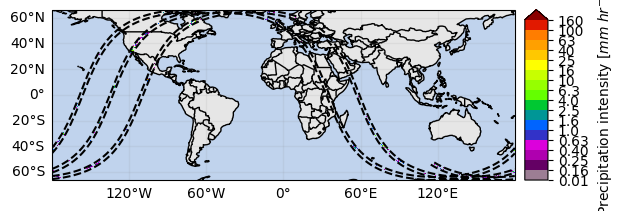
You can customize the map projection by passing a cartopy.crs.Projection to the subplot. The available projections are listed here.
[ ]:
# Define some figure options
dpi = 100
figsize = (12, 10)

# Example of Cartopy projections
crs_proj = ccrs.Robinson()

# Select a single variable
da = ds[variable]

# Create the map
fig, ax = plt.subplots(subplot_kw={"projection": crs_proj}, figsize=figsize, dpi=dpi)
da.gpm.plot_map(ax=ax, add_labels=False, add_background=True, add_gridlines=False, add_swath_lines=True)
ax.set_global()
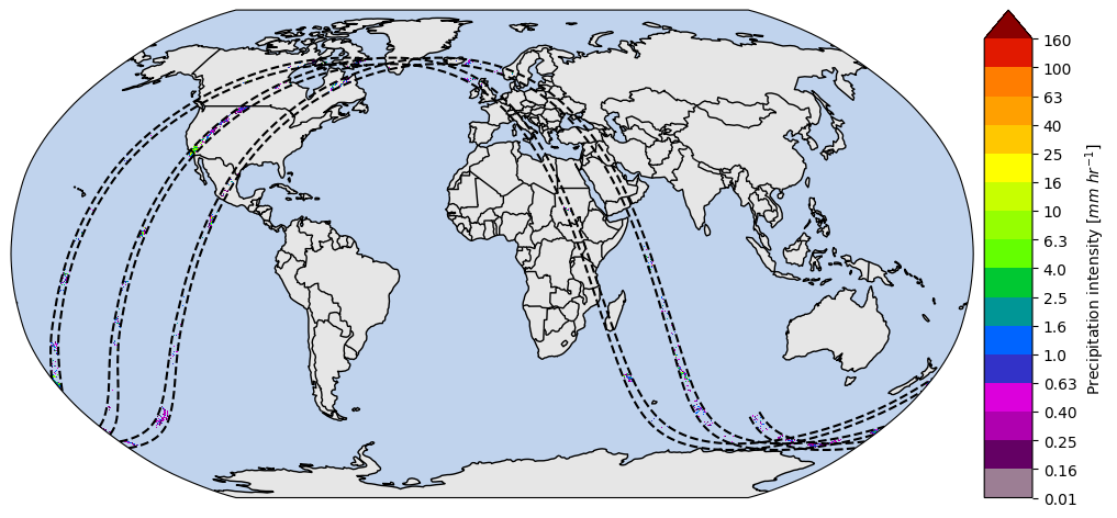
By focusing on a narrow region, it’s possible to better visualize the spatial field:
[ ]:
p = ds[variable].gpm.sel(gpm_id=slice(start_gpm_id, end_gpm_id)).gpm.plot_map()
p.axes.set_title(ds[variable].gpm.title(add_timestep=False))
Text(0.5, 1.0, '2A-DPR PrecipRateNearSurface')
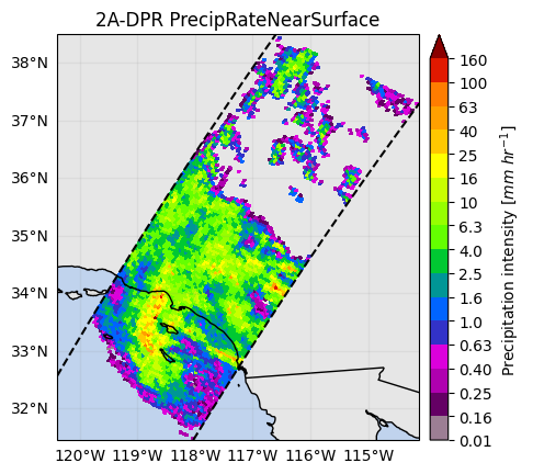
Using the gpm.plot_image method is possible to visualize the data in the so-called “swath scan view”:
[ ]:
ds[variable].gpm.plot_image()
<matplotlib.image.AxesImage at 0x7fd1d0459850>
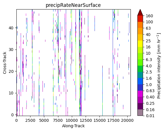
[ ]:
ds[variable].gpm.sel(gpm_id=slice(start_gpm_id, end_gpm_id)).gpm.plot_image()
<matplotlib.image.AxesImage at 0x7fd1f3b60dd0>
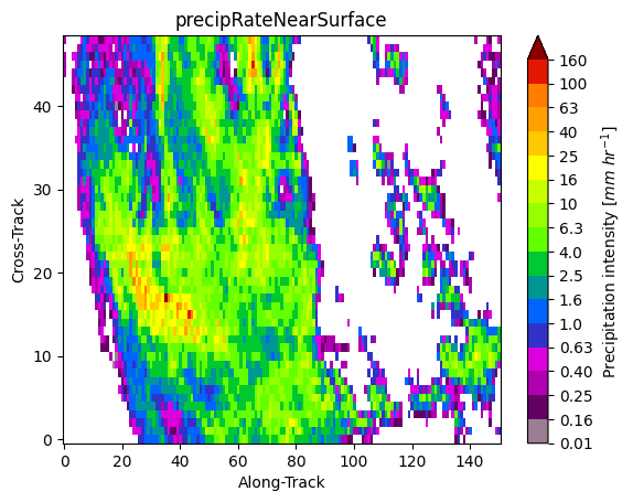
When we visualize different product variables, GPM-API will automatically try to use different appropriate colormaps and colorbars. You can observe this in the following example:
[ ]:
ds_subset = ds.gpm.sel(gpm_id=slice(start_gpm_id, end_gpm_id), radar_frequency="Ku")
ds_subset["zFactorFinalNearSurface"].gpm.plot_map()
ds_subset["zFactorFinalNearSurface"].gpm.plot_map(
    cmap="RdYlBu_r",
    vmin=15,
    vmax=45,
)  # ex: enable to modify defaults parameters on the fly
ds_subset["flagPrecip"].gpm.plot_map()  # ex: defaults to categorical colorbar
<cartopy.mpl.geocollection.GeoQuadMesh at 0x7fd1b4dfe4d0>

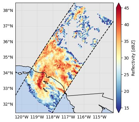
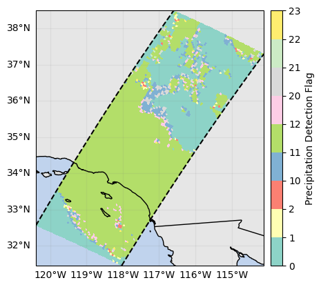
GPM-API provides colormaps and colorbars tailored to GPM product variables with the goal of simplifying the data analysis and make it more reproducible.
The default colormap and colorbar configurations are defined into YAML files into the gpm/etc/colorbars directory of the software.
However, users are free to override, add and/or customize the colorbars configurations using the pycolorbar registry.
The registered colorbar configurations can be displayed using gpm.colorbars.show_colorbars() and the plot_kwargs and cbar_kwargs required to customize the figure can be obtained by calling the gpm.get_plot_kwargs function. Here below we provide an example on how to display DPR precipitation rates estimates using the same colorbar used by NASA to display IMERG liquid precipitation estimates.
[ ]:
plot_kwargs, cbar_kwargs = gpm.get_plot_kwargs("IMERG_Liquid")
ds_subset["precipRateNearSurface"].gpm.plot_map(cbar_kwargs=cbar_kwargs, **plot_kwargs)
<cartopy.mpl.geocollection.GeoQuadMesh at 0x7fd1d0c47110>
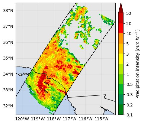
Since GPM Datasets are characterized by multiple dimensions, GPM-API provides the capabilities to generate FacetGrid Cartopy plots following the classical xarray syntax:
[ ]:
ds_subset = ds.gpm.sel(gpm_id=slice(start_gpm_id, end_gpm_id))

# Plot reflectivity at various levels
variable = "zFactorFinal"
da = ds_subset[variable].sel(range=[100, 125, 150, 170])
fc = da.gpm.plot_map(row="radar_frequency", col="range")

# Surface reflectivity at Ku and Ka band
variable = "zFactorFinalNearSurface"
da = ds_subset[variable]
fc = da.gpm.plot_map(col="radar_frequency", col_wrap=2)
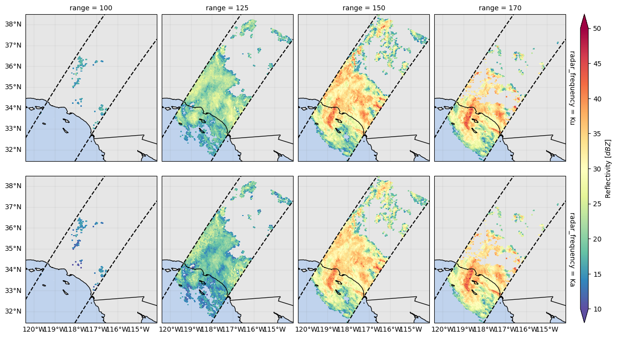
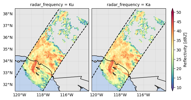
5. Plot Cross-Sections#
An easy way to derive a vertical cross-section is to slice the data along the cross-track or along-track dimension. We can then plot the cross-section calling the gpm.plot_cross_section() method.
[ ]:
ds_subset = ds.gpm.sel(
    gpm_id=slice(start_gpm_id, end_gpm_id),
    radar_frequency="Ku",
).compute()
ds_subset["zFactorFinal"].isel(cross_track=24).gpm.plot_cross_section(zoom=True)
ds_subset["zFactorFinal"].isel(along_track=30).gpm.plot_cross_section(
    y="height_km",
    x="horizontal_distance_km",
    zoom=True,
)
<matplotlib.collections.QuadMesh at 0x7fd1b44fb390>
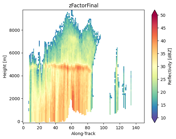
The cross-section transect can be visualized calling the gpm.plot_transect_line method:
[ ]:
ds_transect = ds_subset.isel(cross_track=24)
text_kwargs = {
    "bbox": {
        "facecolor": "white",
        "alpha": 0.6,
        "edgecolor": "black",
        "boxstyle": "round,pad=0.2",
    },
}
p = ds_subset["zFactorFinalNearSurface"].gpm.plot_map()
ds_transect.gpm.plot_transect_line(ax=p.axes, text_kwargs=text_kwargs)
<matplotlib.lines.Line2D at 0x7fd1f0b7a250>
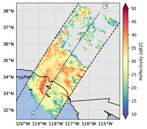
The cross-section variables available in a transect dataset can be listed or selected with gpm.cross_section_variables or gpm.select_cross_section_variables() respectively:
[ ]:
ds_transect = ds_subset.isel(cross_track=24)
print(ds_transect.gpm.cross_section_variables)
ds_transect.gpm.select_cross_section_variables()
['DFRforward1', 'Dm', 'Nw', 'airTemperature', 'attenuationNP', 'dBNw', 'epsilon', 'flagEcho', 'flagSLV', 'phase', 'precipRate', 'precipWater', 'zFactorFinal', 'zFactorMeasured']
<xarray.Dataset> Size: 2MB
Dimensions:             (along_track: 151, range: 176)
Coordinates: (12/15)
    sunLocalTime        (along_track) float32 604B 14.2 14.2 ... 14.48 14.48
    height              (along_track, range) float32 106kB 2.193e+04 ... 29.45
    dataQuality         (along_track) float32 604B 0.0 0.0 0.0 ... 0.0 0.0 0.0
    SCorientation       (along_track) float32 604B 0.0 0.0 0.0 ... 0.0 0.0 0.0
    lon                 (along_track) float32 604B -119.2 -119.2 ... -115.4
    lat                 (along_track) float32 604B 32.04 32.08 ... 37.85 37.89
    ...                  ...
    gpm_cross_track_id  int64 8B 24
    gpm_along_track_id  (along_track) int64 1kB 2768 2769 2770 ... 2917 2918
  * range               (range) int64 1kB 1 2 3 4 5 6 ... 172 173 174 175 176
    gpm_range_id        (range) int64 1kB 0 1 2 3 4 5 ... 171 172 173 174 175
    radar_frequency     <U2 8B 'Ku'
    crsWGS84            int64 8B 0
Dimensions without coordinates: along_track
Data variables: (12/14)
    DFRforward1         (along_track, range) float32 106kB nan nan ... nan nan
    Dm                  (along_track, range) float32 106kB nan nan ... nan nan
    Nw                  (along_track, range) float32 106kB nan nan ... nan nan
    airTemperature      (along_track, range) float32 106kB 214.1 213.9 ... 299.4
    attenuationNP       (along_track, range) float32 106kB 0.0 0.0 ... 0.04
    dBNw                (along_track, range) float32 106kB nan nan ... nan nan
    ...                  ...
    flagSLV             (along_track, range) float32 106kB 0.0 0.0 ... -64.0
    phase               (along_track, range) float32 106kB nan nan ... nan nan
    precipRate          (along_track, range) float32 106kB 0.0 0.0 ... nan nan
    precipWater         (along_track, range) float32 106kB 0.0 0.0 ... nan nan
    zFactorFinal        (along_track, range) float32 106kB nan nan ... nan nan
    zFactorMeasured     (along_track, range) float32 106kB nan nan ... nan 10.78
Attributes: (12/23)
    FileName:              2A.GPM.DPR.V9-20211125.20230820-S183436-E200708.05...
    EphemerisFileName:
    AttitudeFileName:
    TotalQualityCode:      Good
    DielectricFactorKa:    0.8989
    DielectricFactorKu:    0.9255
    ...                    ...
    DataFormatVersion:     7h
    MetadataVersion:       7h
    ProcessingMode:        STD
    ScanMode:              FS
    history:               Created by ghiggi/gpm_api software on 2025-03-01 2...
gpm_api_product: 2A-DPR- along_track: 151
- range: 176
- sunLocalTime(along_track)float3214.2 14.2 14.2 ... 14.48 14.48
- units :
- decimal hours
- source_dtype :
- float32
- gpm_api_product :
- 2A-DPR
- grid_mapping :
- crsWGS84
array([14.198227 , 14.2 , 14.201774 , 14.20355 , 14.205328 , 14.207106 , 14.208887 , 14.210669 , 14.212452 , 14.214238 , 14.216023 , 14.217813 , 14.219602 , 14.221393 , 14.2231865, 14.22498 , 14.226776 , 14.228574 , 14.230372 , 14.232174 , 14.233976 , 14.23578 , 14.237585 , 14.239392 , 14.2412 , 14.243011 , 14.2448225, 14.246636 , 14.248451 , 14.250268 , 14.252087 , 14.253906 , 14.255728 , 14.257551 , 14.259376 , 14.261202 , 14.26303 , 14.264859 , 14.266691 , 14.268524 , 14.270358 , 14.272196 , 14.274033 , 14.275873 , 14.277715 , 14.279557 , 14.281403 , 14.283249 , 14.285096 , 14.286947 , 14.288798 , 14.290651 , 14.292507 , 14.294363 , 14.296222 , 14.298081 , 14.299943 , 14.301806 , 14.303672 , 14.305538 , 14.307407 , 14.309277 , 14.31115 , 14.313024 , 14.3148985, 14.316776 , 14.318655 , 14.320536 , 14.322419 , 14.324303 , 14.326189 , 14.328077 , 14.329966 , 14.331859 , 14.333751 , 14.335646 , 14.337543 , 14.33944 , 14.341341 , 14.343244 , 14.345147 , 14.347054 , 14.34896 , 14.350869 , 14.352781 , 14.354693 , 14.356608 , 14.358525 , 14.360442 , 14.362364 , 14.364285 , 14.366209 , 14.368135 , 14.370063 , 14.371993 , 14.373924 , 14.375857 , 14.377793 , 14.37973 , 14.381669 , 14.383611 , 14.385552 , 14.387498 , 14.389444 , 14.391393 , 14.393344 , 14.395295 , 14.397249 , 14.399206 , 14.401163 , 14.403124 , 14.405086 , 14.407049 , 14.409016 , 14.410983 , 14.412952 , 14.414925 , 14.416898 , 14.418874 , 14.420852 , 14.422831 , 14.424813 , 14.426797 , 14.4287815, 14.430771 , 14.432759 , 14.4347515, 14.436746 , 14.438741 , 14.440739 , 14.442739 , 14.44474 , 14.446745 , 14.44875 , 14.450758 , 14.452768 , 14.45478 , 14.456795 , 14.45881 , 14.460828 , 14.462849 , 14.46487 , 14.466894 , 14.468922 , 14.470949 , 14.47298 , 14.475013 , 14.477046 , 14.479084 , 14.481122 , 14.483163 ], dtype=float32) - height(along_track, range)float322.193e+04 2.18e+04 ... 154.6 29.45
- units :
- m
- source_dtype :
- float32
- gpm_api_product :
- 2A-DPR
- grid_mapping :
- crsWGS84
array([[2.1925812e+04, 2.1800650e+04, 2.1675488e+04, ..., 2.7259937e+02, 1.4743629e+02, 2.2273205e+01], [2.1935410e+04, 2.1810250e+04, 2.1685086e+04, ..., 2.8219781e+02, 1.5703471e+02, 3.1871630e+01], [2.1945113e+04, 2.1819951e+04, 2.1694787e+04, ..., 2.9189954e+02, 1.6673647e+02, 4.1573368e+01], ..., [2.1915096e+04, 2.1789934e+04, 2.1664771e+04, ..., 2.6188287e+02, 1.3671977e+02, 1.1556679e+01], [2.1924289e+04, 2.1799127e+04, 2.1673965e+04, ..., 2.7107620e+02, 1.4591313e+02, 2.0750036e+01], [2.1932986e+04, 2.1807824e+04, 2.1682660e+04, ..., 2.7977377e+02, 1.5461066e+02, 2.9447569e+01]], dtype=float32) - dataQuality(along_track)float320.0 0.0 0.0 0.0 ... 0.0 0.0 0.0 0.0
- source_dtype :
- int8
- gpm_api_product :
- 2A-DPR
array([0., 0., 0., 0., 0., 0., 0., 0., 0., 0., 0., 0., 0., 0., 0., 0., 0., 0., 0., 0., 0., 0., 0., 0., 0., 0., 0., 0., 0., 0., 0., 0., 0., 0., 0., 0., 0., 0., 0., 0., 0., 0., 0., 0., 0., 0., 0., 0., 0., 0., 0., 0., 0., 0., 0., 0., 0., 0., 0., 0., 0., 0., 0., 0., 0., 0., 0., 0., 0., 0., 0., 0., 0., 0., 0., 0., 0., 0., 0., 0., 0., 0., 0., 0., 0., 0., 0., 0., 0., 0., 0., 0., 0., 0., 0., 0., 0., 0., 0., 0., 0., 0., 0., 0., 0., 0., 0., 0., 0., 0., 0., 0., 0., 0., 0., 0., 0., 0., 0., 0., 0., 0., 0., 0., 0., 0., 0., 0., 0., 0., 0., 0., 0., 0., 0., 0., 0., 0., 0., 0., 0., 0., 0., 0., 0., 0., 0., 0., 0., 0., 0.], dtype=float32) - SCorientation(along_track)float320.0 0.0 0.0 0.0 ... 0.0 0.0 0.0 0.0
- units :
- degrees
- source_dtype :
- int16
- gpm_api_product :
- 2A-DPR
array([0., 0., 0., 0., 0., 0., 0., 0., 0., 0., 0., 0., 0., 0., 0., 0., 0., 0., 0., 0., 0., 0., 0., 0., 0., 0., 0., 0., 0., 0., 0., 0., 0., 0., 0., 0., 0., 0., 0., 0., 0., 0., 0., 0., 0., 0., 0., 0., 0., 0., 0., 0., 0., 0., 0., 0., 0., 0., 0., 0., 0., 0., 0., 0., 0., 0., 0., 0., 0., 0., 0., 0., 0., 0., 0., 0., 0., 0., 0., 0., 0., 0., 0., 0., 0., 0., 0., 0., 0., 0., 0., 0., 0., 0., 0., 0., 0., 0., 0., 0., 0., 0., 0., 0., 0., 0., 0., 0., 0., 0., 0., 0., 0., 0., 0., 0., 0., 0., 0., 0., 0., 0., 0., 0., 0., 0., 0., 0., 0., 0., 0., 0., 0., 0., 0., 0., 0., 0., 0., 0., 0., 0., 0., 0., 0., 0., 0., 0., 0., 0., 0.], dtype=float32) - lon(along_track)float32-119.2 -119.2 ... -115.4 -115.4
- name :
- longitude
- standard_name :
- longitude
- long_name :
- longitude
- units :
- degrees_east
- valid_min :
- -180.0
- valid_max :
- 180.0
- comment :
- Geographical coordinates, WGS84 datum
- coverage_content_type :
- coordinate
array([-119.189705, -119.16602 , -119.142334, -119.11861 , -119.094864, -119.071106, -119.0473 , -119.0235 , -118.999664, -118.97579 , -118.95193 , -118.92801 , -118.90408 , -118.88014 , -118.856155, -118.83216 , -118.80814 , -118.78409 , -118.76003 , -118.73593 , -118.711815, -118.687675, -118.663506, -118.63932 , -118.61511 , -118.590866, -118.56662 , -118.54232 , -118.51801 , -118.49369 , -118.46932 , -118.44495 , -118.42055 , -118.39611 , -118.37166 , -118.34718 , -118.32267 , -118.29816 , -118.27359 , -118.24902 , -118.22442 , -118.19978 , -118.17514 , -118.15045 , -118.12574 , -118.10102 , -118.076256, -118.05148 , -118.02669 , -118.00184 , -117.977 , -117.95211 , -117.92719 , -117.902275, -117.877304, -117.85233 , -117.827324, -117.802284, -117.77723 , -117.752144, -117.72703 , -117.701904, -117.67673 , -117.65154 , -117.626335, -117.601074, -117.57582 , -117.55052 , -117.52519 , -117.499855, -117.47447 , -117.44907 , -117.42365 , -117.398186, -117.37272 , -117.34721 , -117.32167 , -117.29613 , -117.27053 , -117.24491 , -117.21928 , -117.193596, -117.167915, -117.14219 , -117.11643 , -117.09067 , -117.06486 , -117.039024, -117.01318 , -116.98728 , -116.96138 , -116.93543 , -116.909454, -116.88347 , -116.85743 , -116.83137 , -116.8053 , -116.779175, -116.75304 , -116.726875, -116.70067 , -116.67445 , -116.64819 , -116.62191 , -116.595604, -116.56925 , -116.54289 , -116.5165 , -116.49007 , -116.46363 , -116.43714 , -116.41063 , -116.384094, -116.35751 , -116.33092 , -116.3043 , -116.277626, -116.25095 , -116.22423 , -116.19747 , -116.1707 , -116.14388 , -116.11705 , -116.090195, -116.06328 , -116.03636 , -116.0094 , -115.9824 , -115.9554 , -115.92834 , -115.90125 , -115.87415 , -115.847 , -115.81984 , -115.79264 , -115.7654 , -115.73815 , -115.710846, -115.683525, -115.65618 , -115.628784, -115.60137 , -115.57393 , -115.54644 , -115.51895 , -115.4914 , -115.46383 , -115.43623 , -115.408585, -115.38093 , -115.35324 ], dtype=float32) - lat(along_track)float3232.04 32.08 32.12 ... 37.85 37.89
- name :
- latitude
- standard_name :
- latitude
- long_name :
- latitude
- units :
- degrees_north
- valid_min :
- -90.0
- valid_max :
- 90.0
- comment :
- Geographical coordinates, WGS84 datum
- coverage_content_type :
- coordinate
array([32.04448 , 32.083946, 32.12337 , 32.162815, 32.202267, 32.24167 , 32.281105, 32.32052 , 32.359917, 32.39934 , 32.43872 , 32.47811 , 32.517513, 32.556866, 32.596256, 32.635624, 32.674965, 32.714344, 32.753677, 32.793015, 32.832375, 32.871677, 32.911015, 32.950333, 32.989624, 33.028954, 33.068237, 33.10752 , 33.146824, 33.186077, 33.22536 , 33.26463 , 33.303867, 33.343147, 33.382385, 33.421623, 33.460884, 33.500095, 33.539333, 33.57856 , 33.61775 , 33.65698 , 33.696163, 33.735348, 33.774555, 33.813705, 33.85289 , 33.892067, 33.931206, 33.970387, 34.00953 , 34.048664, 34.087826, 34.126934, 34.166065, 34.205196, 34.244278, 34.283405, 34.32249 , 34.361572, 34.400677, 34.439735, 34.47881 , 34.517883, 34.55691 , 34.595978, 34.635006, 34.674023, 34.713078, 34.752075, 34.791096, 34.83012 , 34.8691 , 34.908115, 34.947098, 34.98606 , 35.025055, 35.064003, 35.10296 , 35.14193 , 35.180847, 35.2198 , 35.258728, 35.29763 , 35.336563, 35.37545 , 35.41435 , 35.453255, 35.49211 , 35.531006, 35.569878, 35.60872 , 35.647602, 35.686428, 35.72527 , 35.764122, 35.802925, 35.841766, 35.88058 , 35.91937 , 35.95819 , 35.99697 , 36.035748, 36.074547, 36.113293, 36.15207 , 36.190834, 36.22956 , 36.26833 , 36.30705 , 36.34577 , 36.38451 , 36.423195, 36.46191 , 36.50061 , 36.539276, 36.57798 , 36.616642, 36.6553 , 36.69398 , 36.732605, 36.77126 , 36.8099 , 36.8485 , 36.887142, 36.925743, 36.964336, 37.002953, 37.04151 , 37.080097, 37.118675, 37.15721 , 37.19579 , 37.234325, 37.27285 , 37.31141 , 37.349915, 37.38844 , 37.42696 , 37.465435, 37.503944, 37.54242 , 37.58088 , 37.61937 , 37.657803, 37.696255, 37.73471 , 37.773117, 37.811565, 37.849983, 37.888382], dtype=float32) - time(along_track)datetime64[ns]2023-08-20T22:12:00 ... 2023-08-...
- standard_name :
- time
- coverage_content_type :
- coordinate
- axis :
- T
array(['2023-08-20T22:12:00.000000000', '2023-08-20T22:12:01.000000000', '2023-08-20T22:12:01.000000000', '2023-08-20T22:12:02.000000000', '2023-08-20T22:12:03.000000000', '2023-08-20T22:12:04.000000000', '2023-08-20T22:12:04.000000000', '2023-08-20T22:12:05.000000000', '2023-08-20T22:12:06.000000000', '2023-08-20T22:12:06.000000000', '2023-08-20T22:12:07.000000000', '2023-08-20T22:12:08.000000000', '2023-08-20T22:12:08.000000000', '2023-08-20T22:12:09.000000000', '2023-08-20T22:12:10.000000000', '2023-08-20T22:12:11.000000000', '2023-08-20T22:12:11.000000000', '2023-08-20T22:12:12.000000000', '2023-08-20T22:12:13.000000000', '2023-08-20T22:12:13.000000000', '2023-08-20T22:12:14.000000000', '2023-08-20T22:12:15.000000000', '2023-08-20T22:12:15.000000000', '2023-08-20T22:12:16.000000000', '2023-08-20T22:12:17.000000000', '2023-08-20T22:12:18.000000000', '2023-08-20T22:12:18.000000000', '2023-08-20T22:12:19.000000000', '2023-08-20T22:12:20.000000000', '2023-08-20T22:12:20.000000000', '2023-08-20T22:12:21.000000000', '2023-08-20T22:12:22.000000000', '2023-08-20T22:12:22.000000000', '2023-08-20T22:12:23.000000000', '2023-08-20T22:12:24.000000000', '2023-08-20T22:12:25.000000000', '2023-08-20T22:12:25.000000000', '2023-08-20T22:12:26.000000000', '2023-08-20T22:12:27.000000000', '2023-08-20T22:12:27.000000000', ... '2023-08-20T22:13:18.000000000', '2023-08-20T22:13:19.000000000', '2023-08-20T22:13:20.000000000', '2023-08-20T22:13:21.000000000', '2023-08-20T22:13:21.000000000', '2023-08-20T22:13:22.000000000', '2023-08-20T22:13:23.000000000', '2023-08-20T22:13:23.000000000', '2023-08-20T22:13:24.000000000', '2023-08-20T22:13:25.000000000', '2023-08-20T22:13:25.000000000', '2023-08-20T22:13:26.000000000', '2023-08-20T22:13:27.000000000', '2023-08-20T22:13:28.000000000', '2023-08-20T22:13:28.000000000', '2023-08-20T22:13:29.000000000', '2023-08-20T22:13:30.000000000', '2023-08-20T22:13:30.000000000', '2023-08-20T22:13:31.000000000', '2023-08-20T22:13:32.000000000', '2023-08-20T22:13:32.000000000', '2023-08-20T22:13:33.000000000', '2023-08-20T22:13:34.000000000', '2023-08-20T22:13:35.000000000', '2023-08-20T22:13:35.000000000', '2023-08-20T22:13:36.000000000', '2023-08-20T22:13:37.000000000', '2023-08-20T22:13:37.000000000', '2023-08-20T22:13:38.000000000', '2023-08-20T22:13:39.000000000', '2023-08-20T22:13:39.000000000', '2023-08-20T22:13:40.000000000', '2023-08-20T22:13:41.000000000', '2023-08-20T22:13:42.000000000', '2023-08-20T22:13:42.000000000', '2023-08-20T22:13:43.000000000', '2023-08-20T22:13:44.000000000', '2023-08-20T22:13:44.000000000', '2023-08-20T22:13:45.000000000'], dtype='datetime64[ns]') - gpm_id(along_track)<U10'53847-2768' ... '53847-2918'
- long_name :
- Scan ID
- description :
- Scan ID. Format: '{gpm_granule_id}-{gpm_along_track_id}'
- coverage_content_type :
- auxiliaryInformation
array(['53847-2768', '53847-2769', '53847-2770', '53847-2771', '53847-2772', '53847-2773', '53847-2774', '53847-2775', '53847-2776', '53847-2777', '53847-2778', '53847-2779', '53847-2780', '53847-2781', '53847-2782', '53847-2783', '53847-2784', '53847-2785', '53847-2786', '53847-2787', '53847-2788', '53847-2789', '53847-2790', '53847-2791', '53847-2792', '53847-2793', '53847-2794', '53847-2795', '53847-2796', '53847-2797', '53847-2798', '53847-2799', '53847-2800', '53847-2801', '53847-2802', '53847-2803', '53847-2804', '53847-2805', '53847-2806', '53847-2807', '53847-2808', '53847-2809', '53847-2810', '53847-2811', '53847-2812', '53847-2813', '53847-2814', '53847-2815', '53847-2816', '53847-2817', '53847-2818', '53847-2819', '53847-2820', '53847-2821', '53847-2822', '53847-2823', '53847-2824', '53847-2825', '53847-2826', '53847-2827', '53847-2828', '53847-2829', '53847-2830', '53847-2831', '53847-2832', '53847-2833', '53847-2834', '53847-2835', '53847-2836', '53847-2837', '53847-2838', '53847-2839', '53847-2840', '53847-2841', '53847-2842', '53847-2843', '53847-2844', '53847-2845', '53847-2846', '53847-2847', '53847-2848', '53847-2849', '53847-2850', '53847-2851', '53847-2852', '53847-2853', '53847-2854', '53847-2855', '53847-2856', '53847-2857', '53847-2858', '53847-2859', '53847-2860', '53847-2861', '53847-2862', '53847-2863', '53847-2864', '53847-2865', '53847-2866', '53847-2867', '53847-2868', '53847-2869', '53847-2870', '53847-2871', '53847-2872', '53847-2873', '53847-2874', '53847-2875', '53847-2876', '53847-2877', '53847-2878', '53847-2879', '53847-2880', '53847-2881', '53847-2882', '53847-2883', '53847-2884', '53847-2885', '53847-2886', '53847-2887', '53847-2888', '53847-2889', '53847-2890', '53847-2891', '53847-2892', '53847-2893', '53847-2894', '53847-2895', '53847-2896', '53847-2897', '53847-2898', '53847-2899', '53847-2900', '53847-2901', '53847-2902', '53847-2903', '53847-2904', '53847-2905', '53847-2906', '53847-2907', '53847-2908', '53847-2909', '53847-2910', '53847-2911', '53847-2912', '53847-2913', '53847-2914', '53847-2915', '53847-2916', '53847-2917', '53847-2918'], dtype='<U10') - gpm_granule_id(along_track)int6453847 53847 53847 ... 53847 53847
- long_name :
- GPM Granule ID
- description :
- ID number of the GPM Granule
- coverage_content_type :
- auxiliaryInformation
array([53847, 53847, 53847, 53847, 53847, 53847, 53847, 53847, 53847, 53847, 53847, 53847, 53847, 53847, 53847, 53847, 53847, 53847, 53847, 53847, 53847, 53847, 53847, 53847, 53847, 53847, 53847, 53847, 53847, 53847, 53847, 53847, 53847, 53847, 53847, 53847, 53847, 53847, 53847, 53847, 53847, 53847, 53847, 53847, 53847, 53847, 53847, 53847, 53847, 53847, 53847, 53847, 53847, 53847, 53847, 53847, 53847, 53847, 53847, 53847, 53847, 53847, 53847, 53847, 53847, 53847, 53847, 53847, 53847, 53847, 53847, 53847, 53847, 53847, 53847, 53847, 53847, 53847, 53847, 53847, 53847, 53847, 53847, 53847, 53847, 53847, 53847, 53847, 53847, 53847, 53847, 53847, 53847, 53847, 53847, 53847, 53847, 53847, 53847, 53847, 53847, 53847, 53847, 53847, 53847, 53847, 53847, 53847, 53847, 53847, 53847, 53847, 53847, 53847, 53847, 53847, 53847, 53847, 53847, 53847, 53847, 53847, 53847, 53847, 53847, 53847, 53847, 53847, 53847, 53847, 53847, 53847, 53847, 53847, 53847, 53847, 53847, 53847, 53847, 53847, 53847, 53847, 53847, 53847, 53847, 53847, 53847, 53847, 53847, 53847, 53847]) - gpm_cross_track_id()int6424
- long_name :
- Cross-Track ID
- description :
- Cross-Track ID.
- coverage_content_type :
- auxiliaryInformation
array(24)
- gpm_along_track_id(along_track)int642768 2769 2770 ... 2916 2917 2918
- long_name :
- Along-Track ID
- description :
- Along-Track ID.
- coverage_content_type :
- auxiliaryInformation
array([2768, 2769, 2770, 2771, 2772, 2773, 2774, 2775, 2776, 2777, 2778, 2779, 2780, 2781, 2782, 2783, 2784, 2785, 2786, 2787, 2788, 2789, 2790, 2791, 2792, 2793, 2794, 2795, 2796, 2797, 2798, 2799, 2800, 2801, 2802, 2803, 2804, 2805, 2806, 2807, 2808, 2809, 2810, 2811, 2812, 2813, 2814, 2815, 2816, 2817, 2818, 2819, 2820, 2821, 2822, 2823, 2824, 2825, 2826, 2827, 2828, 2829, 2830, 2831, 2832, 2833, 2834, 2835, 2836, 2837, 2838, 2839, 2840, 2841, 2842, 2843, 2844, 2845, 2846, 2847, 2848, 2849, 2850, 2851, 2852, 2853, 2854, 2855, 2856, 2857, 2858, 2859, 2860, 2861, 2862, 2863, 2864, 2865, 2866, 2867, 2868, 2869, 2870, 2871, 2872, 2873, 2874, 2875, 2876, 2877, 2878, 2879, 2880, 2881, 2882, 2883, 2884, 2885, 2886, 2887, 2888, 2889, 2890, 2891, 2892, 2893, 2894, 2895, 2896, 2897, 2898, 2899, 2900, 2901, 2902, 2903, 2904, 2905, 2906, 2907, 2908, 2909, 2910, 2911, 2912, 2913, 2914, 2915, 2916, 2917, 2918]) - range(range)int641 2 3 4 5 6 ... 172 173 174 175 176
array([ 1, 2, 3, 4, 5, 6, 7, 8, 9, 10, 11, 12, 13, 14, 15, 16, 17, 18, 19, 20, 21, 22, 23, 24, 25, 26, 27, 28, 29, 30, 31, 32, 33, 34, 35, 36, 37, 38, 39, 40, 41, 42, 43, 44, 45, 46, 47, 48, 49, 50, 51, 52, 53, 54, 55, 56, 57, 58, 59, 60, 61, 62, 63, 64, 65, 66, 67, 68, 69, 70, 71, 72, 73, 74, 75, 76, 77, 78, 79, 80, 81, 82, 83, 84, 85, 86, 87, 88, 89, 90, 91, 92, 93, 94, 95, 96, 97, 98, 99, 100, 101, 102, 103, 104, 105, 106, 107, 108, 109, 110, 111, 112, 113, 114, 115, 116, 117, 118, 119, 120, 121, 122, 123, 124, 125, 126, 127, 128, 129, 130, 131, 132, 133, 134, 135, 136, 137, 138, 139, 140, 141, 142, 143, 144, 145, 146, 147, 148, 149, 150, 151, 152, 153, 154, 155, 156, 157, 158, 159, 160, 161, 162, 163, 164, 165, 166, 167, 168, 169, 170, 171, 172, 173, 174, 175, 176]) - gpm_range_id(range)int640 1 2 3 4 5 ... 171 172 173 174 175
array([ 0, 1, 2, 3, 4, 5, 6, 7, 8, 9, 10, 11, 12, 13, 14, 15, 16, 17, 18, 19, 20, 21, 22, 23, 24, 25, 26, 27, 28, 29, 30, 31, 32, 33, 34, 35, 36, 37, 38, 39, 40, 41, 42, 43, 44, 45, 46, 47, 48, 49, 50, 51, 52, 53, 54, 55, 56, 57, 58, 59, 60, 61, 62, 63, 64, 65, 66, 67, 68, 69, 70, 71, 72, 73, 74, 75, 76, 77, 78, 79, 80, 81, 82, 83, 84, 85, 86, 87, 88, 89, 90, 91, 92, 93, 94, 95, 96, 97, 98, 99, 100, 101, 102, 103, 104, 105, 106, 107, 108, 109, 110, 111, 112, 113, 114, 115, 116, 117, 118, 119, 120, 121, 122, 123, 124, 125, 126, 127, 128, 129, 130, 131, 132, 133, 134, 135, 136, 137, 138, 139, 140, 141, 142, 143, 144, 145, 146, 147, 148, 149, 150, 151, 152, 153, 154, 155, 156, 157, 158, 159, 160, 161, 162, 163, 164, 165, 166, 167, 168, 169, 170, 171, 172, 173, 174, 175]) - radar_frequency()<U2'Ku'
array('Ku', dtype='<U2') - crsWGS84()int640
- crs_wkt :
- GEOGCRS["unknown",DATUM["Unknown based on WGS 84 ellipsoid",ELLIPSOID["WGS 84",6378137,298.257223563,LENGTHUNIT["metre",1],ID["EPSG",7030]]],PRIMEM["Greenwich",0,ANGLEUNIT["degree",0.0174532925199433],ID["EPSG",8901]],CS[ellipsoidal,2],AXIS["longitude",east,ORDER[1],ANGLEUNIT["degree",0.0174532925199433,ID["EPSG",9122]]],AXIS["latitude",north,ORDER[2],ANGLEUNIT["degree",0.0174532925199433,ID["EPSG",9122]]]]
- semi_major_axis :
- 6378137.0
- semi_minor_axis :
- 6356752.314245179
- inverse_flattening :
- 298.257223563
- reference_ellipsoid_name :
- WGS 84
- longitude_of_prime_meridian :
- 0.0
- prime_meridian_name :
- Greenwich
- geographic_crs_name :
- unknown
- horizontal_datum_name :
- Unknown based on WGS 84 ellipsoid
- grid_mapping_name :
- latitude_longitude
- spatial_ref :
- GEOGCS["unknown",DATUM["Unknown based on WGS 84 ellipsoid",ELLIPSOID["WGS 84",6378137,298.257223563,LENGTHUNIT["metre",1],ID["EPSG",7030]]],PRIMEM["Greenwich",0,ANGLEUNIT["degree",0.0174532925199433],ID["EPSG",8901]],CS[ellipsoidal,2],AXIS["longitude",east,ORDER[1],ANGLEUNIT["degree",0.0174532925199433,ID["EPSG",9122]]],AXIS["latitude",north,ORDER[2],ANGLEUNIT["degree",0.0174532925199433,ID["EPSG",9122]]]]
array(0)
- DFRforward1(along_track, range)float32nan nan nan nan ... nan nan nan nan
- gpm_api_product :
- 2A-DPR
- grid_mapping :
- crsWGS84
array([[nan, nan, nan, ..., nan, nan, nan], [nan, nan, nan, ..., nan, nan, nan], [nan, nan, nan, ..., nan, nan, nan], ..., [nan, nan, nan, ..., nan, nan, nan], [nan, nan, nan, ..., nan, nan, nan], [nan, nan, nan, ..., nan, nan, nan]], dtype=float32) - Dm(along_track, range)float32nan nan nan nan ... nan nan nan nan
- gpm_api_product :
- 2A-DPR
- units :
- mm
- long_name :
- Mass weighted mean diameter
- gpm_api_decoded :
- yes
- grid_mapping :
- crsWGS84
array([[nan, nan, nan, ..., nan, nan, nan], [nan, nan, nan, ..., nan, nan, nan], [nan, nan, nan, ..., nan, nan, nan], ..., [nan, nan, nan, ..., nan, nan, nan], [nan, nan, nan, ..., nan, nan, nan], [nan, nan, nan, ..., nan, nan, nan]], dtype=float32) - Nw(along_track, range)float32nan nan nan nan ... nan nan nan nan
- units :
- 1/(mm*m^3)
- gpm_api_decoded :
- yes
- grid_mapping :
- crsWGS84
array([[nan, nan, nan, ..., nan, nan, nan], [nan, nan, nan, ..., nan, nan, nan], [nan, nan, nan, ..., nan, nan, nan], ..., [nan, nan, nan, ..., nan, nan, nan], [nan, nan, nan, ..., nan, nan, nan], [nan, nan, nan, ..., nan, nan, nan]], dtype=float32) - airTemperature(along_track, range)float32214.1 213.9 213.7 ... 299.1 299.4
- units :
- K
- gpm_api_product :
- 2A-DPR
- grid_mapping :
- crsWGS84
array([[214.08786, 213.88095, 213.67404, ..., 292.559 , 292.8935 , 293.22525], [214.11993, 213.91248, 213.70502, ..., 292.5867 , 292.91315, 293.2396 ], [214.15123, 213.94318, 213.73512, ..., 292.61462, 292.93362, 293.2526 ], ..., [215.12985, 214.92795, 214.72603, ..., 298.5537 , 299.1744 , 299.2618 ], [215.1553 , 214.95314, 214.75098, ..., 298.53946, 299.15973, 299.33423], [215.17969, 214.9774 , 214.77512, ..., 298.52423, 299.14404, 299.4004 ]], dtype=float32) - attenuationNP(along_track, range)float320.0 0.0 0.0 ... 0.038 0.039 0.04
- units :
- dB/km
- gpm_api_product :
- 2A-DPR
- gpm_api_decoded :
- yes
- grid_mapping :
- crsWGS84
array([[0. , 0. , 0. , ..., 0.029, 0.03 , 0.031], [0. , 0. , 0. , ..., 0.029, 0.03 , 0.031], [0. , 0. , 0. , ..., 0.029, 0.03 , 0.031], ..., [0. , 0. , 0. , ..., 0.038, 0.04 , 0.04 ], [0. , 0. , 0. , ..., 0.038, 0.04 , 0.04 ], [0. , 0. , 0. , ..., 0.038, 0.039, 0.04 ]], dtype=float32) - dBNw(along_track, range)float32nan nan nan nan ... nan nan nan nan
- gpm_api_product :
- 2A-DPR
- units :
- 10log10(1/(mm*m^3))
- gpm_api_decoded :
- yes
- grid_mapping :
- crsWGS84
array([[nan, nan, nan, ..., nan, nan, nan], [nan, nan, nan, ..., nan, nan, nan], [nan, nan, nan, ..., nan, nan, nan], ..., [nan, nan, nan, ..., nan, nan, nan], [nan, nan, nan, ..., nan, nan, nan], [nan, nan, nan, ..., nan, nan, nan]], dtype=float32) - epsilon(along_track, range)float32nan nan nan nan ... nan nan nan nan
- gpm_api_product :
- 2A-DPR
- grid_mapping :
- crsWGS84
array([[nan, nan, nan, ..., nan, nan, nan], [nan, nan, nan, ..., nan, nan, nan], [nan, nan, nan, ..., nan, nan, nan], ..., [nan, nan, nan, ..., nan, nan, nan], [nan, nan, nan, ..., nan, nan, nan], [nan, nan, nan, ..., nan, nan, nan]], dtype=float32) - flagEcho(along_track, range)float320.0 0.0 0.0 0.0 ... 48.0 48.0 48.0
- gpm_api_product :
- 2A-DPR
- grid_mapping :
- crsWGS84
array([[ 0., 0., 0., ..., 48., 48., 48.], [ 0., 0., 0., ..., 48., 48., 48.], [ 0., 0., 0., ..., 48., 48., 48.], ..., [ 0., 0., 0., ..., 48., 48., 48.], [ 0., 0., 0., ..., 48., 48., 48.], [ 0., 0., 0., ..., 48., 48., 48.]], dtype=float32) - flagSLV(along_track, range)float320.0 0.0 0.0 ... -64.0 -64.0 -64.0
- gpm_api_product :
- 2A-DPR
- grid_mapping :
- crsWGS84
array([[ 0., 0., 0., ..., 0., 0., 0.], [ 0., 0., 0., ..., 0., 0., 0.], [ 0., 0., 0., ..., 0., 0., 0.], ..., [ 0., 0., 0., ..., -64., -64., -64.], [ 0., 0., 0., ..., -64., -64., -64.], [ 0., 0., 0., ..., -64., -64., -64.]], dtype=float32) - phase(along_track, range)float32nan nan nan nan ... nan nan nan nan
- gpm_api_product :
- 2A-DPR
- flag_values :
- [0, 1, 2]
- flag_meanings :
- ['solid', 'mixed_phase', 'liquid']
- description :
- Precipitation Phase State
- gpm_api_decoded :
- yes
- grid_mapping :
- crsWGS84
array([[nan, nan, nan, ..., nan, nan, nan], [nan, nan, nan, ..., nan, nan, nan], [nan, nan, nan, ..., nan, nan, nan], ..., [nan, nan, nan, ..., nan, nan, nan], [nan, nan, nan, ..., nan, nan, nan], [nan, nan, nan, ..., nan, nan, nan]], dtype=float32) - precipRate(along_track, range)float320.0 0.0 0.0 0.0 ... nan nan nan nan
- units :
- mm/hr
- gpm_api_product :
- 2A-DPR
- grid_mapping :
- crsWGS84
array([[ 0., 0., 0., ..., 0., 0., 0.], [ 0., 0., 0., ..., 0., 0., 0.], [ 0., 0., 0., ..., 0., 0., 0.], ..., [ 0., 0., 0., ..., nan, nan, nan], [ 0., 0., 0., ..., nan, nan, nan], [ 0., 0., 0., ..., nan, nan, nan]], dtype=float32) - precipWater(along_track, range)float320.0 0.0 0.0 0.0 ... nan nan nan nan
- units :
- kg/m^3
- gpm_api_product :
- 2A-DPR
- grid_mapping :
- crsWGS84
array([[ 0., 0., 0., ..., 0., 0., 0.], [ 0., 0., 0., ..., 0., 0., 0.], [ 0., 0., 0., ..., 0., 0., 0.], ..., [ 0., 0., 0., ..., nan, nan, nan], [ 0., 0., 0., ..., nan, nan, nan], [ 0., 0., 0., ..., nan, nan, nan]], dtype=float32) - zFactorFinal(along_track, range)float32nan nan nan nan ... nan nan nan nan
- units :
- dBZ
- gpm_api_product :
- 2A-DPR
- grid_mapping :
- crsWGS84
array([[nan, nan, nan, ..., nan, nan, nan], [nan, nan, nan, ..., nan, nan, nan], [nan, nan, nan, ..., nan, nan, nan], ..., [nan, nan, nan, ..., nan, nan, nan], [nan, nan, nan, ..., nan, nan, nan], [nan, nan, nan, ..., nan, nan, nan]], dtype=float32) - zFactorMeasured(along_track, range)float32nan nan nan nan ... 8.86 nan 10.78
- units :
- dBZ
- gpm_api_product :
- 2A-DPR
- gpm_api_decoded :
- yes
- grid_mapping :
- crsWGS84
array([[  nan,   nan,   nan, ..., 25.33, 49.02, 57.89],
       [  nan,   nan,   nan, ..., 25.07, 48.95, 57.1 ],
       [  nan,   nan,   nan, ..., 25.48, 49.95, 60.06],
       ...,
       [  nan,   nan,   nan, ..., 10.73, 10.79,   nan],
       [  nan,   nan,   nan, ..., 11.61,  9.97,   nan],
       [  nan,   nan,   nan, ...,  8.86,   nan, 10.78]], dtype=float32)
- rangePandasIndex
PandasIndex(Index([  1,   2,   3,   4,   5,   6,   7,   8,   9,  10,
       ...
       167, 168, 169, 170, 171, 172, 173, 174, 175, 176],
      dtype='int64', name='range', length=176))
- FileName :
- 2A.GPM.DPR.V9-20211125.20230820-S183436-E200708.053845.V07B.HDF5
- EphemerisFileName :
- AttitudeFileName :
- TotalQualityCode :
- Good
- DielectricFactorKa :
- 0.8989
- DielectricFactorKu :
- 0.9255
- MissingData :
- 0
- NumberOfRainPixelsFS :
- 23568
- NumberOfRainPixelsHS :
- 0
- DOI :
- 10.5067/GPM/DPR/GPM/2A/07
- DOIauthority :
- http://dx.doi.org/
- AlgorithmID :
- 2ADPR
- AlgorithmVersion :
- 9.20211125
- ProductVersion :
- V07B
- SatelliteName :
- GPM
- InstrumentName :
- DPR
- ProcessingSystem :
- PPS
- DataFormatVersion :
- 7h
- MetadataVersion :
- 7h
- ProcessingMode :
- STD
- ScanMode :
- FS
- history :
- Created by ghiggi/gpm_api software on 2025-03-01 20:10:24
- gpm_api_product :
- 2A-DPR
GPM-API provides accessor methods to facilitate the extraction of cross-section: - around a point - between points - and along a trajectory.
[ ]:
da_cross = ds_subset["zFactorFinal"].gpm.extract_transect_between_points(
    start_point=(-118, 32),
    end_point=(-118, 36),
    steps=60,
)
da_cross.gpm.plot_cross_section(zoom=True)
<matplotlib.collections.QuadMesh at 0x7fd1f0ac1090>
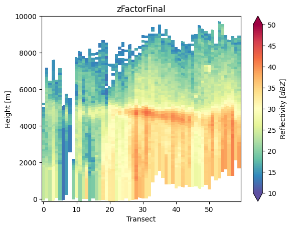
[ ]:
points = np.ones((100, 2))
points[:, 0] = -118
points[:, 1] = np.linspace(32, 36, 100)
da_cross = ds_subset["zFactorFinal"].gpm.extract_transect_at_points(points=points)
da_cross.gpm.plot_cross_section(zoom=True)
<matplotlib.collections.QuadMesh at 0x7fd1b45cd190>
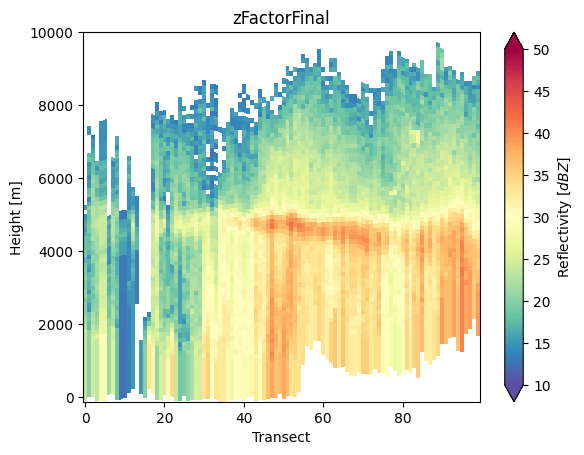
[ ]:
da_cross = ds_subset["zFactorFinal"].gpm.extract_transect_around_point(
    point=(-118, 34),
    azimuth=0,
    distance=100_000,
    steps=100,
)  # azimuth [0, 360]
da_cross.gpm.plot_cross_section(zoom=True)
<matplotlib.collections.QuadMesh at 0x7fd1f0bcec90>
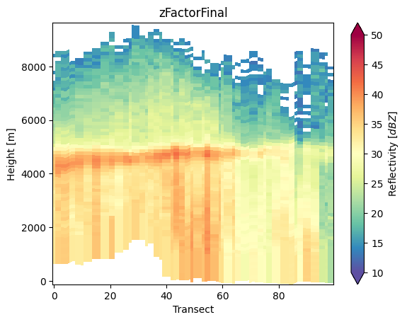
6. Community-based retrievals#
GPM-API aims to be a platform where scientist can share their algorithms and retrievals with the community.
Based on the GPM product you are working with, you will have a series of retrievals available to you. For example, GPM-API currently provides the following retrievals for the 2A-DPR product:
[ ]:
ds.gpm.available_retrievals()
['EchoDepth',
 'EchoTopHeight',
 'HailKineticEnergy',
 'MESH',
 'MESHS',
 'POH',
 'POSH',
 'REFC',
 'REFCH',
 'SHI',
 'VIL',
 'VILD',
 'bright_band_ratio',
 'c_band_tan',
 'dfrFinal',
 'dfrFinalNearSurface',
 'dfrMeasured',
 'flagHydroClass',
 'flagPrecipitationType',
 'gate_resolution',
 'gate_volume',
 'heightClutterFreeBottom',
 'heightRealSurfaceKa',
 'heightRealSurfaceKu',
 'range_distance_from_ellipsoid',
 'range_distance_from_satellite',
 'range_resolution',
 's_band_cao2013',
 'x_band_tan']
The gpm.retrieve method enables you to apply specific retrievals to your dataset. Here below we provide a couple of examples:
[ ]:
ds_subset = ds.gpm.sel(
    gpm_id=slice(start_gpm_id, end_gpm_id),
    radar_frequency="Ku",
).compute()

ds_subset["EchoTopHeight40dBZ"] = ds_subset.gpm.retrieve("EchoTopHeight", threshold=40)
ds_subset["EchoTopHeight40dBZ"].gpm.plot_map()
<cartopy.mpl.geocollection.GeoQuadMesh at 0x7fd1f0db1190>
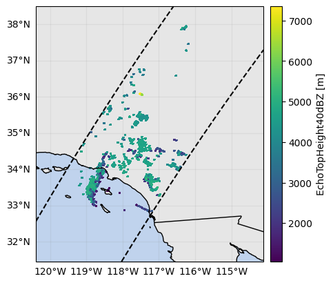
[ ]:
ds_subset["EchoDepthSolid30dBZ"] = ds_subset.gpm.retrieve(
    "EchoDepth",
    threshold=30,
    mask_liquid_phase=True,
)
ds_subset["EchoDepthSolid30dBZ"].gpm.plot_map()
<cartopy.mpl.geocollection.GeoQuadMesh at 0x7fd1f08a9dd0>
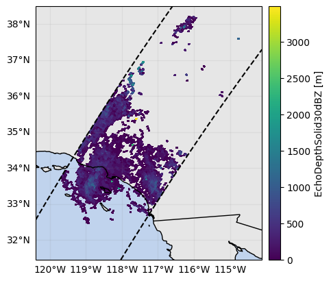
[ ]:
ds_subset["flagPrecipitationType"] = ds_subset.gpm.retrieve(
    "flagPrecipitationType",
    method="major_rain_type",
)
ds_subset["flagPrecipitationType"].gpm.plot_map()
<cartopy.mpl.geocollection.GeoQuadMesh at 0x7fd1b4d4e810>
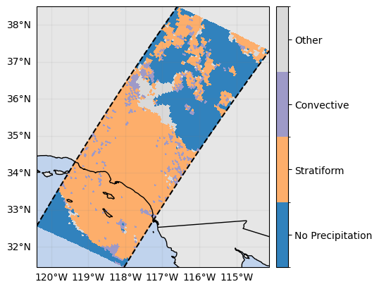
[ ]:
ds_subset["flagHydroClass"] = ds_subset.gpm.retrieve(
    "flagHydroClass",
)  # this return a 3D array !
ds_subset["flagHydroClass"].isel(cross_track=24).gpm.plot_cross_section()
<matplotlib.collections.QuadMesh at 0x7fd1d0b09c90>
7. Advanced Manipulations#
When working with spaceborne radar data, it is often necessary to slice, extract or mask portions of data across the range dimension. The xarray gpm accessor provides a series of methods to facilitate various tasks.
If you wish to extract the values at specific range gate position varying over each radar beam, you can use the slice_range_at_bin method. For example, to extract values near the surface where radar gates are not more contaminated by ground clutter, you can use the bin variable "binClutterFreeBottom":
[ ]:
ds_surface = ds_subset.gpm.slice_range_at_bin(
    bins="binClutterFreeBottom",
)  # or ds.gpm.slice_range_at_bin(bins=ds["binClutterFreeBottom"])
ds_surface["precipRate"].gpm.plot_map()  # precipRate is originally a 3D variable !
ds_surface["zFactorFinal"].gpm.plot_map()  # zFactorFinal is originally a 3D variable !
<cartopy.mpl.geocollection.GeoQuadMesh at 0x7fd2222b1d50>
Other slicing methods provide capabilities to retrieve values at a given height, along isothermals, or at the range gates where the minimum, maximum or closest value of a given variable occur:
[ ]:
ds_isothermal = ds_subset.gpm.slice_range_at_temperature(
    273.15,
)  # use by default the airTemperature variable
ds_3000 = ds_subset.gpm.slice_range_at_height(3000)
ds_max_z = ds_subset.gpm.slice_range_at_max_value(variable="zFactorFinal")
ds_min_z = ds_subset.gpm.slice_range_at_min_value(variable="zFactorFinal")
ds_at_z_30 = ds_subset.gpm.slice_range_at_value(variable="zFactorFinal", value=30)
If you want to focus your analysis in the portion of radar gates with valid values (e.g., excluding upper atmosphere regions without reflectivities) or values ranging in a specific interval of interest, you can use the subset_range_with_valid_data and subset_range_where_values methods respectively:
[ ]:
ds_valid = ds_subset.gpm.subset_range_with_valid_data(variable="zFactorFinal")
ds_intense = ds_subset.gpm.subset_range_where_values(
    variable="precipRate",
    vmin=200,
    vmax=300,
)  # mm/hr
print("Range with valid data:", ds_valid["range"].data)
print("Range with intense precipitation:", ds_intense["range"].data)
Range with valid data: [ 93  94  95  96  97  98  99 100 101 102 103 104 105 106 107 108 109 110
 111 112 113 114 115 116 117 118 119 120 121 122 123 124 125 126 127 128
 129 130 131 132 133 134 135 136 137 138 139 140 141 142 143 144 145 146
 147 148 149 150 151 152 153 154 155 156 157 158 159 160 161 162 163 164
 165 166 167 168 169 170 171 172 173 174 175 176]
Range with intense precipitation: [166 167 168 169 170 171 172 173 174 175 176]
If you wish to extract radar gates above/below spatially-varying bin position, you can use the extract_dataset_above_bin and extract_dataset_below_bin methods. Please note that these methods shifts the arrays beam-wise, returning datasets with a new range coordinate and the bin variables updated accordingly.
[ ]:
ds_below_melting_layer = ds_subset.gpm.extract_dataset_below_bin(
    "binBBBottom",
)  # the first new range index corresponds to original binBBBottom
ds_above_melting_layer = ds_subset.gpm.extract_dataset_above_bin(
    "binBBTop",
)  # the last new range index corresponds to original binBBTop
If instead you wish to mask the data above/below or in between radar gates positions, you can use the mask_above_bin, mask_below_bin and mask_between_bins methods:
[ ]:
ds_rain = ds_subset.gpm.mask_above_bin("binZeroDeg")
ds_snow = ds_subset.gpm.mask_below_bin("binZeroDeg")
ds_masked_melting_layer = ds_subset.gpm.mask_between_bins(
    bottom_bins="binBBBottom",
    top_bins="binBBTop",
)
8. Geospatial Manipulations#
GPM-API provides methods to easily spatially subset orbits by extent, country or continent.
Note however, that an area can be crossed by multiple orbits depending on the size of your GPM satellite dataset. In other words, multiple orbit slices in along-track direction can intersect the area of interest.
The method get_crop_slices_by_extent, get_crop_slices_by_country and get_crop_slices_by_continent enable to retrieve the orbit portions intersecting the area of interest.
[ ]:
# Define the variable to display
variable = "precipRateNearSurface"

# Crop by country
list_isel_dict = ds.gpm.get_crop_slices_by_country("United States")
print(list_isel_dict)

# Crop by extent
extent = get_country_extent("United States")
list_isel_dict = ds.gpm.get_crop_slices_by_extent(extent)
print(list_isel_dict)

# Plot the swaths crossing the country
for isel_dict in list_isel_dict:
    da_subset = ds[variable].isel(isel_dict)
    slice_title = da_subset.gpm.title(add_timestep=True)
    p = da_subset.gpm.plot_map()
    p.axes.set_extent(extent)
    p.axes.set_title(label=slice_title)
[{'along_track': slice(3040, 4143, None)}, {'along_track': slice(10973, 12352, None)}, {'along_track': slice(18905, 20509, None)}]
[{'along_track': slice(3040, 4143, None)}, {'along_track': slice(10973, 12352, None)}, {'along_track': slice(18905, 20509, None)}]
Alternatively, if yourare working with a single granule, you can use the following methods:
[ ]:
# ds_subset = ds.gpm.crop(extent)
# ds_subset = ds.gpm.crop_by_country("United States")
You can also easily obtain the extent around a given point (i.e. ground radar location) using the get_geographic_extent_around_point function and use the gpm accessor methods get_crop_slices_around_point or crop_around_point to subset your dataset:
[ ]:
# Define the variable to display
variable = "precipRateNearSurface"

# Crop around a point (i.e. radar location)
lon = -117.0418
lat = 32.9190
distance = 200_000  # 200 km
list_isel_dict = ds.gpm.get_crop_slices_around_point(
    lon=lon,
    lat=lat,
    distance=distance,
)
print(list_isel_dict)

extent = get_geographic_extent_around_point(lon=lon, lat=lat, distance=distance)
list_isel_dict = ds.gpm.get_crop_slices_by_extent(extent)
print(list_isel_dict)

# Define ROI coordinates
circle_lons, circle_lats = get_circle_coordinates_around_point(
    lon,
    lat,
    radius=distance,
    num_vertices=360,
)

# Plot the swaths crossing the ROI
for isel_dict in list_isel_dict:
    da_subset = ds[variable].isel(isel_dict)
    slice_title = da_subset.gpm.title(add_timestep=True)
    p = da_subset.gpm.plot_map()
    p.axes.set_title(slice_title)
    p.axes.plot(circle_lons, circle_lats, "r-", transform=ccrs.Geodetic())
    p.axes.scatter(lon, lat, c="black", marker="X", s=100, transform=ccrs.Geodetic())
    p.axes.set_extent(extent)

# Alternatives if working with a single granule:

# ds_subset = ds.gpm.crop_around_point(lon=lon, lat=lat, distance=distance)
[{'along_track': slice(11298, 11399, None)}]
[{'along_track': slice(11298, 11399, None)}]
Please keep in mind that you can easily retrieve the extent of a GPM xarray object using the extent method.
The optional argument padding allows to expand/shrink the geographic extent by custom lon/lat degrees, while the size argument allows to obtain an extent centered on the GPM object with the desired size.
[ ]:
print(da_subset.gpm.extent(padding=0.1))  # expanding
print(da_subset.gpm.extent(padding=-0.1))  # shrinking
print(da_subset.gpm.extent(size=0.5))
print(da_subset.gpm.extent(size=0))  # centroid
Extent(xmin=-120.85270843505859, xmax=-115.86820831298829, ymin=30.720465087890624, ymax=35.94685516357422)
Extent(xmin=-120.6527084350586, xmax=-116.06820831298828, ymin=30.920465087890626, ymax=35.74685516357422)
Extent(xmin=-118.61045837402344, xmax=-118.11045837402344, ymin=33.08366012573242, ymax=33.58366012573242)
Extent(xmin=-118.36045837402344, xmax=-118.36045837402344, ymin=33.33366012573242, ymax=33.33366012573242)
9. Storm Labeling#
Using the xarray ximage accessor, it is possible to easily delineate (label) the precipitating areas. The label array is added to the dataset as a new coordinate.
[ ]:
# Retrieve labeled xarray object
label_name = "label"
ds = ds.ximage.label(
    variable="precipRateNearSurface",
    min_value_threshold=1,
    min_area_threshold=5,
    footprint=5,  # assign same label to precipitating areas 5 pixels apart
    sort_by="area",  # "maximum", "minimum", <custom_function>
    sort_decreasing=True,
    label_name=label_name,
)
# Plot full label array
ds[label_name].ximage.plot_labels()
The array currently contains 121 labels and 'max_n_labels'
            is set to 50. The colorbar is not displayed!
<matplotlib.image.AxesImage at 0x7fd1b40f52d0>
Let’s zoom in a specific region:
[ ]:
gpm.plot_labels(ds[label_name].isel(along_track=slice(2700, 3500)))
<matplotlib.image.AxesImage at 0x7fd1a3f4d810>
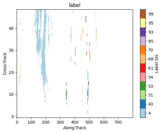
10. Patch Extraction#
With the xarray ximage accessor, it is also possible to extract patches around the precipitating areas. Here we provide a minimal example on how to proceed:
[ ]:
# Define the patch generator
da_patch_gen = ds["precipRateNearSurface"].ximage.label_patches(
    label_name=label_name,
    patch_size=(49, 49),
    # Output options
    n_patches=4,
    # Patch extraction Options
    padding=0,
    centered_on="max",
    # Tiling/Sliding Options
    debug=False,
    verbose=False,
)

# # Retrieve list of patches
list_label_patches = list(da_patch_gen)
list_da = [da for label, da in list_label_patches]

# Display patches
gpm.plot_patches(list_label_patches)
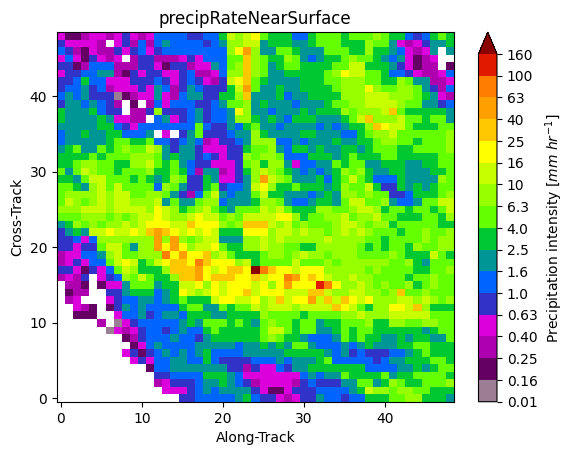
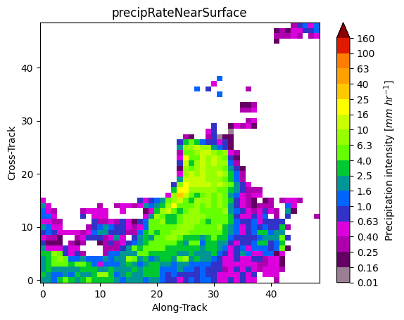
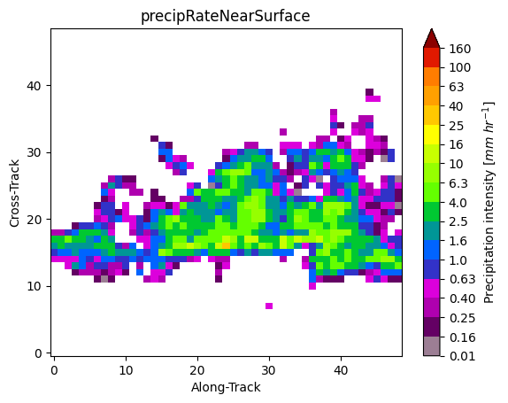
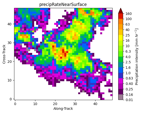
You can exploit the xarray manipulations and FacetGrid capabilities to quickly create the following figure:
[ ]:
list_da_without_coords = [da.drop_vars(["lon", "lat"]) for da in list_da]
da_patch = xr.concat(list_da_without_coords, dim="patch")
da_patch.isel(patch=slice(0, 4)).gpm.plot_image(col="patch", col_wrap=2)
<gpm.visualization.facetgrid.ImageFacetGrid at 0x7fd1b426cd90>