PMW 2A products#
In this tutorial, we will provide the foundations to use GPM-API to download, manipulate and analyze data from the Global Precipitation Measurement (GPM) Passive Microwave (PMW) 2A products.
Please note that GPM-API also enable access and analysis tools for the entire GPM constellation of passive microwave sensors as well as the IMERG precipitation products. For detailed information and additional tutorials, please refer to the others GPM-API tutorials.
First, let’s import the package required in this tutorial.
[ ]:
import datetime

import cartopy.crs as ccrs
import matplotlib.pyplot as plt
import xarray as xr
import ximage  # noqa

import gpm
from gpm.utils.geospatial import (
    get_circle_coordinates_around_point,
    get_country_extent,
    get_geographic_extent_around_point,
)
Using the available_products function, users can obtain a list of all GPM products that can be downloaded and opened into CF-compliant xarray datasets.
[ ]:
gpm.available_products(product_types="RS") # research products
['1A-GMI',
 '1A-TMI',
 '1B-GMI',
 '1B-Ka',
 '1B-Ku',
 '1B-PR',
 '1B-TMI',
 '1C-AMSR2-GCOMW1',
 '1C-AMSRE-AQUA',
 '1C-AMSUB-NOAA15',
 '1C-AMSUB-NOAA16',
 '1C-AMSUB-NOAA17',
 '1C-ATMS-NOAA20',
 '1C-ATMS-NOAA21',
 '1C-ATMS-NPP',
 '1C-GMI',
 '1C-GMI-R',
 '1C-MHS-METOPA',
 '1C-MHS-METOPB',
 '1C-MHS-METOPC',
 '1C-MHS-NOAA18',
 '1C-MHS-NOAA19',
 '1C-SAPHIR-MT1',
 '1C-SSMI-F08',
 '1C-SSMI-F10',
 '1C-SSMI-F11',
 '1C-SSMI-F13',
 '1C-SSMI-F14',
 '1C-SSMI-F15',
 '1C-SSMIS-F16',
 '1C-SSMIS-F17',
 '1C-SSMIS-F18',
 '1C-SSMIS-F19',
 '1C-TMI',
 '2A-AMSR2-GCOMW1',
 '2A-AMSR2-GCOMW1-CLIM',
 '2A-AMSRE-AQUA-CLIM',
 '2A-AMSUB-NOAA15-CLIM',
 '2A-AMSUB-NOAA16-CLIM',
 '2A-AMSUB-NOAA17-CLIM',
 '2A-ATMS-NOAA20',
 '2A-ATMS-NOAA20-CLIM',
 '2A-ATMS-NOAA21',
 '2A-ATMS-NOAA21-CLIM',
 '2A-ATMS-NPP',
 '2A-ATMS-NPP-CLIM',
 '2A-DPR',
 '2A-ENV-DPR',
 '2A-ENV-Ka',
 '2A-ENV-Ku',
 '2A-ENV-PR',
 '2A-GMI',
 '2A-GMI-CLIM',
 '2A-GPM-SLH',
 '2A-Ka',
 '2A-Ku',
 '2A-MHS-METOPA',
 '2A-MHS-METOPA-CLIM',
 '2A-MHS-METOPB',
 '2A-MHS-METOPB-CLIM',
 '2A-MHS-METOPC',
 '2A-MHS-METOPC-CLIM',
 '2A-MHS-NOAA18',
 '2A-MHS-NOAA18-CLIM',
 '2A-MHS-NOAA19',
 '2A-MHS-NOAA19-CLIM',
 '2A-PR',
 '2A-SAPHIR-MT1',
 '2A-SAPHIR-MT1-CLIM',
 '2A-SSMI-F08-CLIM',
 '2A-SSMI-F10-CLIM',
 '2A-SSMI-F11-CLIM',
 '2A-SSMI-F13-CLIM',
 '2A-SSMI-F14-CLIM',
 '2A-SSMI-F15-CLIM',
 '2A-SSMIS-F16',
 '2A-SSMIS-F16-CLIM',
 '2A-SSMIS-F17',
 '2A-SSMIS-F17-CLIM',
 '2A-SSMIS-F18',
 '2A-SSMIS-F18-CLIM',
 '2A-SSMIS-F19',
 '2A-SSMIS-F19-CLIM',
 '2A-TMI-CLIM',
 '2A-TRMM-SLH',
 '2B-GPM-CORRA',
 '2B-GPM-CSAT',
 '2B-GPM-CSH',
 '2B-TRMM-CORRA',
 '2B-TRMM-CSAT',
 '2B-TRMM-CSH',
 'IMERG-FR']
Let’s have a look at the available PMW 2A products:
[ ]:
gpm.available_products(product_categories="PMW", product_levels="2A")
['2A-AMSR2-GCOMW1',
 '2A-AMSR2-GCOMW1-CLIM',
 '2A-AMSRE-AQUA-CLIM',
 '2A-AMSUB-NOAA15-CLIM',
 '2A-AMSUB-NOAA16-CLIM',
 '2A-AMSUB-NOAA17-CLIM',
 '2A-ATMS-NOAA20',
 '2A-ATMS-NOAA20-CLIM',
 '2A-ATMS-NOAA21',
 '2A-ATMS-NOAA21-CLIM',
 '2A-ATMS-NPP',
 '2A-ATMS-NPP-CLIM',
 '2A-GMI',
 '2A-GMI-CLIM',
 '2A-MHS-METOPA',
 '2A-MHS-METOPA-CLIM',
 '2A-MHS-METOPB',
 '2A-MHS-METOPB-CLIM',
 '2A-MHS-METOPC',
 '2A-MHS-METOPC-CLIM',
 '2A-MHS-NOAA18',
 '2A-MHS-NOAA18-CLIM',
 '2A-MHS-NOAA19',
 '2A-MHS-NOAA19-CLIM',
 '2A-SAPHIR-MT1',
 '2A-SAPHIR-MT1-CLIM',
 '2A-SSMI-F08-CLIM',
 '2A-SSMI-F10-CLIM',
 '2A-SSMI-F11-CLIM',
 '2A-SSMI-F13-CLIM',
 '2A-SSMI-F14-CLIM',
 '2A-SSMI-F15-CLIM',
 '2A-SSMIS-F16',
 '2A-SSMIS-F16-CLIM',
 '2A-SSMIS-F17',
 '2A-SSMIS-F17-CLIM',
 '2A-SSMIS-F18',
 '2A-SSMIS-F18-CLIM',
 '2A-SSMIS-F19',
 '2A-SSMIS-F19-CLIM',
 '2A-TMI-CLIM']
The CLIM products differ from their ‘regular’ counterparts (without the CLIM in the name) by the ancillary data they use. The CLIM products use the ECMWF-Interim reanalysis data to derive surface and atmospheric conditions required by the GPROF algorithm. The ‘regular’ NRT and RS products use the GANAL forecast and anaylsis respectively.
1. Download Data#
Now let’s download a 2A PMW product over a couple of hours.
To download GPM data with GPM-API, you have to previously create a NASA Earthdata and/or NASA PPS account. We provide a step-by-step guide on how to set up your accounts in the official GPM-API documentation.
[ ]:
# Specify the time period you are interested in
start_time = datetime.datetime.strptime("2020-08-01 12:00:00", "%Y-%m-%d %H:%M:%S")
end_time = datetime.datetime.strptime("2020-08-02 12:00:00", "%Y-%m-%d %H:%M:%S")
# Specify the product and product type
product = "2A-MHS-METOPB-CLIM"  # "2A-GMI-CLIM", "2A-SSMIS-F17-CLIM", ...
product_type = "RS"
storage = "GES_DISC"
# Specify the version
version = 7
[ ]:
# Download the data
gpm.download(
    product=product,
    product_type=product_type,
    version=version,
    start_time=start_time,
    end_time=end_time,
    storage=storage,
    force_download=False,
    verbose=True,
    progress_bar=True,
    check_integrity=False,
)
All the available GPM 2A-MHS-METOPB-CLIM product files are already on disk.
Once, the data are downloaded on disk, let’s load the 2A PMW product and look at the dataset structure.
2. Load Data#
With GPM-API, the name granule is used to refer to a single file, while the name dataset is used to refer to a collection of granules.
GPM-API enables to open single or multiple granules into xarray, a software designed for working with labeled multi-dimensional arrays.
The
gpm.open_granule_dataset(filepath)opens a single granule into axarray.Datasetobject by providing the path of the file of interest.The
gpm.open_datasetfunction enable to open a collection of granules over a period of interest intoxarray.Datasetobject.
[ ]:
ds = gpm.open_dataset(
    product=product,
    product_type=product_type,
    version=version,
    start_time=start_time,
    end_time=end_time,
)
ds
/home/ghiggi/Python_Packages/gpm_api/gpm/dataset/dataset.py:296: GPM_Warning: 'Presence of invalid geolocation coordinates !'
  ds = finalize_dataset(
/home/ghiggi/Python_Packages/gpm_api/gpm/dataset/dataset.py:296: GPM_Warning: 'Presence of non-contiguous scans !'
  ds = finalize_dataset(
<xarray.Dataset> Size: 388MB
Dimensions:                     (cross_track: 90, along_track: 32400,
                                 nspecies: 5)
Coordinates:
    sunLocalTime                (cross_track, along_track) float32 12MB dask.array<chunksize=(90, 237), meta=np.ndarray>
    L1CqualityFlag              (cross_track, along_track) float32 12MB dask.array<chunksize=(90, 237), meta=np.ndarray>
    SCorientation               (along_track) float32 130kB dask.array<chunksize=(237,), meta=np.ndarray>
    lon                         (cross_track, along_track) float32 12MB -32.6...
    lat                         (cross_track, along_track) float32 12MB -53.8...
    time                        (along_track) datetime64[ns] 259kB 2020-08-01...
    gpm_id                      (along_track) <U10 1MB ...
    gpm_granule_id              (along_track) int64 259kB ...
    gpm_cross_track_id          (cross_track) int64 720B ...
    gpm_along_track_id          (along_track) int64 259kB ...
    crsWGS84                    int64 8B 0
Dimensions without coordinates: cross_track, along_track, nspecies
Data variables: (12/25)
    pixelStatus                 (cross_track, along_track) float32 12MB dask.array<chunksize=(90, 237), meta=np.ndarray>
    qualityFlag                 (cross_track, along_track) float32 12MB dask.array<chunksize=(90, 237), meta=np.ndarray>
    surfaceTypeIndex            (cross_track, along_track) float32 12MB dask.array<chunksize=(90, 237), meta=np.ndarray>
    totalColumnWaterVaporIndex  (cross_track, along_track) float32 12MB dask.array<chunksize=(90, 237), meta=np.ndarray>
    airmassLiftIndex            (cross_track, along_track) float32 12MB dask.array<chunksize=(90, 237), meta=np.ndarray>
    temp2mIndex                 (cross_track, along_track) float32 12MB dask.array<chunksize=(90, 237), meta=np.ndarray>
    ...                          ...
    profileNumber               (cross_track, along_track, nspecies) float32 58MB dask.array<chunksize=(90, 237, 5), meta=np.ndarray>
    profileScale                (cross_track, along_track, nspecies) float32 58MB dask.array<chunksize=(90, 237, 5), meta=np.ndarray>
    SClatitude                  (along_track) float32 130kB dask.array<chunksize=(237,), meta=np.ndarray>
    SClongitude                 (along_track) float32 130kB dask.array<chunksize=(237,), meta=np.ndarray>
    SCaltitude                  (along_track) float32 130kB dask.array<chunksize=(237,), meta=np.ndarray>
    FractionalGranuleNumber     (along_track) float64 259kB dask.array<chunksize=(237,), meta=np.ndarray>
Attributes: (12/19)
    FileName:           2A-CLIM.METOPB.MHS.GPROF2021v1.20200801-S102909-E1210...
    EphemerisFileName:
    AttitudeFileName:
    MissingData:        0
    DOI:                10.5067/GPM/MHS/METOPB/GPROFCLIM/2A/07
    DOIauthority:       http://dx.doi.org/
    ...                 ...
    MetadataVersion:    7c
    Satellite:          METOPB
    Sensor:             MHS
    ScanMode:           S1
    history:            Created by ghiggi/gpm_api software on 2025-03-05 20:4...
gpm_api_product: 2A-MHS-METOPB-CLIMIf you are interested to work only with a specific subset of variables, you can specify their names using the variables argument in gpm.open_dataset function.
[ ]:
ds1 = gpm.open_dataset(
    product=product,
    product_type=product_type,
    version=version,
    start_time=start_time,
    end_time=end_time,
    variables=["surfacePrecipitation", "precipitationYesNoFlag"],
)
ds1
/home/ghiggi/Python_Packages/gpm_api/gpm/dataset/dataset.py:296: GPM_Warning: 'Presence of invalid geolocation coordinates !'
  ds = finalize_dataset(
/home/ghiggi/Python_Packages/gpm_api/gpm/dataset/dataset.py:296: GPM_Warning: 'Presence of non-contiguous scans !'
  ds = finalize_dataset(
<xarray.Dataset> Size: 61MB
Dimensions:                 (cross_track: 90, along_track: 32400)
Coordinates:
    L1CqualityFlag          (cross_track, along_track) float32 12MB dask.array<chunksize=(90, 237), meta=np.ndarray>
    SCorientation           (along_track) float32 130kB dask.array<chunksize=(237,), meta=np.ndarray>
    lon                     (cross_track, along_track) float32 12MB -32.6 ......
    lat                     (cross_track, along_track) float32 12MB -53.85 .....
    time                    (along_track) datetime64[ns] 259kB 2020-08-01T12:...
    gpm_id                  (along_track) <U10 1MB ...
    gpm_granule_id          (along_track) int64 259kB ...
    gpm_cross_track_id      (cross_track) int64 720B ...
    gpm_along_track_id      (along_track) int64 259kB ...
    crsWGS84                int64 8B 0
Dimensions without coordinates: cross_track, along_track
Data variables:
    precipitationYesNoFlag  (cross_track, along_track) float32 12MB dask.array<chunksize=(90, 237), meta=np.ndarray>
    surfacePrecipitation    (cross_track, along_track) float32 12MB dask.array<chunksize=(90, 237), meta=np.ndarray>
Attributes: (12/19)
    FileName:           2A-CLIM.METOPB.MHS.GPROF2021v1.20200801-S102909-E1210...
    EphemerisFileName:
    AttitudeFileName:
    MissingData:        0
    DOI:                10.5067/GPM/MHS/METOPB/GPROFCLIM/2A/07
    DOIauthority:       http://dx.doi.org/
    ...                 ...
    MetadataVersion:    7c
    Satellite:          METOPB
    Sensor:             MHS
    ScanMode:           S1
    history:            Created by ghiggi/gpm_api software on 2025-03-05 20:4...
gpm_api_product: 2A-MHS-METOPB-CLIM3. Basic Manipulations#
You can list variables, coordinates and dimensions with the following methods:
[ ]:
# Available variables
variables = list(ds.data_vars)
print("Available variables: ", variables)
# Available coordinates
coords = list(ds.coords)
print("Available coordinates: ", coords)
# Available dimensions
dims = list(ds.dims)
print("Available dimensions: ", dims)
Available variables:  ['pixelStatus', 'qualityFlag', 'surfaceTypeIndex', 'totalColumnWaterVaporIndex', 'airmassLiftIndex', 'temp2mIndex', 'sunGlintAngle', 'probabilityOfPrecip', 'precipitationYesNoFlag', 'surfacePrecipitation', 'frozenPrecipitation', 'convectivePrecipitation', 'rainWaterPath', 'cloudWaterPath', 'iceWaterPath', 'mostLikelyPrecipitation', 'precip1stTertial', 'precip2ndTertial', 'profileTemp2mIndex', 'profileNumber', 'profileScale', 'SClatitude', 'SClongitude', 'SCaltitude', 'FractionalGranuleNumber']
Available coordinates:  ['sunLocalTime', 'L1CqualityFlag', 'SCorientation', 'lon', 'lat', 'time', 'gpm_id', 'gpm_granule_id', 'gpm_cross_track_id', 'gpm_along_track_id', 'crsWGS84']
Available dimensions:  ['cross_track', 'along_track', 'nspecies']
To select the DataArray corresponding to a single variable:
[ ]:
variable = "surfacePrecipitation"
da = ds[variable]
print("Array class: ", type(da.data))
da
Array class: <class 'dask.array.core.Array'>
<xarray.DataArray 'surfacePrecipitation' (cross_track: 90, along_track: 32400)> Size: 12MB
dask.array<getitem, shape=(90, 32400), dtype=float32, chunksize=(90, 2281), chunktype=numpy.ndarray>
Coordinates:
    sunLocalTime        (cross_track, along_track) float32 12MB dask.array<chunksize=(90, 237), meta=np.ndarray>
    L1CqualityFlag      (cross_track, along_track) float32 12MB dask.array<chunksize=(90, 237), meta=np.ndarray>
    SCorientation       (along_track) float32 130kB dask.array<chunksize=(237,), meta=np.ndarray>
    lon                 (cross_track, along_track) float32 12MB -32.6 ... 168.2
    lat                 (cross_track, along_track) float32 12MB -53.85 ... -4...
    time                (along_track) datetime64[ns] 259kB 2020-08-01T12:00:0...
    gpm_id              (along_track) <U10 1MB ...
    gpm_granule_id      (along_track) int64 259kB ...
    gpm_cross_track_id  (cross_track) int64 720B ...
    gpm_along_track_id  (along_track) int64 259kB ...
    crsWGS84            int64 8B 0
Dimensions without coordinates: cross_track, along_track
Attributes:
    units:            mm/hr
    gpm_api_product:  2A-MHS-METOPB-CLIM
    gpm_api_decoded:  yes
grid_mapping: crsWGS84If the array class is dask.Array, it means that the data are not yet loaded into RAM memory. To put the data into memory, you need to call the method compute, either on the xarray object or on the numerical array.
[ ]:
da = da.compute()
print("Array class: ", type(da.data))
da
Array class: <class 'numpy.ndarray'>
<xarray.DataArray 'surfacePrecipitation' (cross_track: 90, along_track: 32400)> Size: 12MB
array([[nan, nan, nan, ..., nan, nan, nan],
       [nan, nan, nan, ..., nan, nan, nan],
       [nan, nan, nan, ..., nan, nan, nan],
       ...,
       [nan, nan, nan, ..., nan, nan, nan],
       [nan, nan, nan, ..., nan, nan, nan],
       [nan, nan, nan, ..., nan, nan, nan]], dtype=float32)
Coordinates:
    sunLocalTime        (cross_track, along_track) float32 12MB 9.722 ... 23.11
    L1CqualityFlag      (cross_track, along_track) float32 12MB 0.0 0.0 ... 0.0
    SCorientation       (along_track) float32 130kB 0.0 0.0 0.0 ... 0.0 0.0 0.0
    lon                 (cross_track, along_track) float32 12MB -32.6 ... 168.2
    lat                 (cross_track, along_track) float32 12MB -53.85 ... -4...
    time                (along_track) datetime64[ns] 259kB 2020-08-01T12:00:0...
    gpm_id              (along_track) <U10 1MB '40841-2044' ... '40856-234'
    gpm_granule_id      (along_track) int64 259kB 40841 40841 ... 40856 40856
    gpm_cross_track_id  (cross_track) int64 720B 0 1 2 3 4 5 ... 85 86 87 88 89
    gpm_along_track_id  (along_track) int64 259kB 2044 2045 2046 ... 232 233 234
    crsWGS84            int64 8B 0
Dimensions without coordinates: cross_track, along_track
Attributes:
    units:            mm/hr
    gpm_api_product:  2A-MHS-METOPB-CLIM
    gpm_api_decoded:  yes
grid_mapping: crsWGS84To extract the numerical array from the xarray.DataArray, you can use:
[ ]:
da.data
array([[nan, nan, nan, ..., nan, nan, nan],
       [nan, nan, nan, ..., nan, nan, nan],
       [nan, nan, nan, ..., nan, nan, nan],
       ...,
       [nan, nan, nan, ..., nan, nan, nan],
       [nan, nan, nan, ..., nan, nan, nan],
       [nan, nan, nan, ..., nan, nan, nan]], dtype=float32)
Since xarray does not yet allow subsetting by value along non-dimensional coordinates, the gpm.sel method provides you this functionality.
As an example, you can subset the dataset by time:
[ ]:
start_time = datetime.datetime.strptime("2020-08-01 22:12:00", "%Y-%m-%d %H:%M:%S")
end_time = datetime.datetime.strptime("2020-08-01 22:14:45", "%Y-%m-%d %H:%M:%S")
ds_subset = ds.gpm.sel(time=slice(start_time, end_time))
ds_subset["time"]
<xarray.DataArray 'time' (along_track: 62)> Size: 496B
array(['2020-08-01T22:12:01.000000000', '2020-08-01T22:12:03.000000000',
       '2020-08-01T22:12:06.000000000', '2020-08-01T22:12:09.000000000',
       '2020-08-01T22:12:11.000000000', '2020-08-01T22:12:14.000000000',
       '2020-08-01T22:12:17.000000000', '2020-08-01T22:12:19.000000000',
       '2020-08-01T22:12:22.000000000', '2020-08-01T22:12:25.000000000',
       '2020-08-01T22:12:27.000000000', '2020-08-01T22:12:30.000000000',
       '2020-08-01T22:12:33.000000000', '2020-08-01T22:12:35.000000000',
       '2020-08-01T22:12:38.000000000', '2020-08-01T22:12:41.000000000',
       '2020-08-01T22:12:43.000000000', '2020-08-01T22:12:46.000000000',
       '2020-08-01T22:12:49.000000000', '2020-08-01T22:12:51.000000000',
       '2020-08-01T22:12:54.000000000', '2020-08-01T22:12:57.000000000',
       '2020-08-01T22:12:59.000000000', '2020-08-01T22:13:02.000000000',
       '2020-08-01T22:13:05.000000000', '2020-08-01T22:13:07.000000000',
       '2020-08-01T22:13:10.000000000', '2020-08-01T22:13:13.000000000',
       '2020-08-01T22:13:15.000000000', '2020-08-01T22:13:18.000000000',
       '2020-08-01T22:13:21.000000000', '2020-08-01T22:13:23.000000000',
       '2020-08-01T22:13:26.000000000', '2020-08-01T22:13:29.000000000',
       '2020-08-01T22:13:31.000000000', '2020-08-01T22:13:34.000000000',
       '2020-08-01T22:13:37.000000000', '2020-08-01T22:13:39.000000000',
       '2020-08-01T22:13:42.000000000', '2020-08-01T22:13:45.000000000',
       '2020-08-01T22:13:47.000000000', '2020-08-01T22:13:50.000000000',
       '2020-08-01T22:13:53.000000000', '2020-08-01T22:13:55.000000000',
       '2020-08-01T22:13:58.000000000', '2020-08-01T22:14:01.000000000',
       '2020-08-01T22:14:03.000000000', '2020-08-01T22:14:06.000000000',
       '2020-08-01T22:14:09.000000000', '2020-08-01T22:14:11.000000000',
       '2020-08-01T22:14:14.000000000', '2020-08-01T22:14:17.000000000',
       '2020-08-01T22:14:19.000000000', '2020-08-01T22:14:22.000000000',
       '2020-08-01T22:14:25.000000000', '2020-08-01T22:14:27.000000000',
       '2020-08-01T22:14:30.000000000', '2020-08-01T22:14:33.000000000',
       '2020-08-01T22:14:35.000000000', '2020-08-01T22:14:38.000000000',
       '2020-08-01T22:14:41.000000000', '2020-08-01T22:14:43.000000000'],
      dtype='datetime64[ns]')
Coordinates:
    SCorientation       (along_track) float32 248B dask.array<chunksize=(62,), meta=np.ndarray>
    time                (along_track) datetime64[ns] 496B 2020-08-01T22:12:01...
    gpm_id              (along_track) <U10 2kB ...
    gpm_granule_id      (along_track) int64 496B ...
    gpm_along_track_id  (along_track) int64 496B ...
    crsWGS84            int64 8B 0
Dimensions without coordinates: along_track
Attributes:
    standard_name:          time
    coverage_content_type:  coordinate
axis: TRemember that you can get the start time and end time of your GPM xarray object with the gpm accessor methods start_time and end_time.
[ ]:
print(ds_subset.gpm.start_time)
print(ds_subset.gpm.end_time)
2020-08-01 22:12:01
2020-08-01 22:14:43
You can also subset your GPM xarray object by gpm_id and gpm_cross_track_id` coordinates, which act as reference identifiers for the along-track, cross-track dimensions. Selecting across coordinates by value is useful for example to: - align multiple GPM xarray objects that might have been subsetted differently across the`cross_track,along_track` dimensions. - to retrieve a specific portion of a GPM granule indipendently of the previous subsetting operations.
The gpm_id is defined as <gpm_granule_number>-<gpm_along_track_id>, while the others <gpm_*_id> coordinates start at 0 and increase incrementally by 1 along each granule dimension.
[ ]:
# Subset by gpm_id
start_gpm_id = "40844-1580"
end_gpm_id = "40844-1699"
ds_subset = ds.gpm.sel(gpm_id=slice(start_gpm_id, end_gpm_id))
ds_subset["gpm_id"].data
array(['40844-1580', '40844-1581', '40844-1582', '40844-1583',
       '40844-1584', '40844-1585', '40844-1586', '40844-1587',
       '40844-1588', '40844-1589', '40844-1590', '40844-1591',
       '40844-1592', '40844-1593', '40844-1594', '40844-1595',
       '40844-1596', '40844-1597', '40844-1598', '40844-1599',
       '40844-1600', '40844-1601', '40844-1602', '40844-1603',
       '40844-1604', '40844-1605', '40844-1606', '40844-1607',
       '40844-1608', '40844-1609', '40844-1610', '40844-1611',
       '40844-1612', '40844-1613', '40844-1614', '40844-1615',
       '40844-1616', '40844-1617', '40844-1618', '40844-1619',
       '40844-1620', '40844-1621', '40844-1622', '40844-1623',
       '40844-1624', '40844-1625', '40844-1626', '40844-1627',
       '40844-1628', '40844-1629', '40844-1630', '40844-1631',
       '40844-1632', '40844-1633', '40844-1634', '40844-1635',
       '40844-1636', '40844-1637', '40844-1638', '40844-1639',
       '40844-1640', '40844-1641', '40844-1642', '40844-1643',
       '40844-1644', '40844-1645', '40844-1646', '40844-1647',
       '40844-1648', '40844-1649', '40844-1650', '40844-1651',
       '40844-1652', '40844-1653', '40844-1654', '40844-1655',
       '40844-1656', '40844-1657', '40844-1658', '40844-1659',
       '40844-1660', '40844-1661', '40844-1662', '40844-1663',
       '40844-1664', '40844-1665', '40844-1666', '40844-1667',
       '40844-1668', '40844-1669', '40844-1670', '40844-1671',
       '40844-1672', '40844-1673', '40844-1674', '40844-1675',
       '40844-1676', '40844-1677', '40844-1678', '40844-1679',
       '40844-1680', '40844-1681', '40844-1682', '40844-1683',
       '40844-1684', '40844-1685', '40844-1686', '40844-1687',
       '40844-1688', '40844-1689', '40844-1690', '40844-1691',
       '40844-1692', '40844-1693', '40844-1694', '40844-1695',
       '40844-1696', '40844-1697', '40844-1698', '40844-1699'],
      dtype='<U10')
To locate the gpm_id where the maximum precipitation occurs, you can for example use the locate_max_value method:
[ ]:
isel_dict = ds["surfacePrecipitation"].gpm.locate_max_value(return_isel_dict=True)
print(isel_dict)
print("gpm_id:", ds.isel(along_track=isel_dict["along_track"])["gpm_id"].values)
{'along_track': 6438, 'cross_track': 24}
gpm_id: 40844-1640
To check whether the GPM 2A-PMW product has contiguous along-track scans (with no missing scans), you can use:
[ ]:
print(ds.gpm.has_contiguous_scans)
print(ds.gpm.is_regular)
False
False
In case there are non-contiguous scans, you can obtain the along-track slices over which the dataset is regular:
[ ]:
list_slices = ds.gpm.get_slices_contiguous_scans()
print(list_slices)
[slice(0, 22204, None), slice(22205, 32400, None)]
You can then select a regular portion of the dataset with:
[ ]:
slc = list_slices[0]
print(slc)
ds_regular = ds.isel(along_track=slc)
slice(0, 22204, None)
4. Plot Maps#
The GPM-API provides two ways of displaying the data:
The
plot_mapmethod plot the data in a geographic projection using the CartopypcolormeshmethodThe
plot_imagemethod plot the data as an image using the Maplotlibimshowmethod
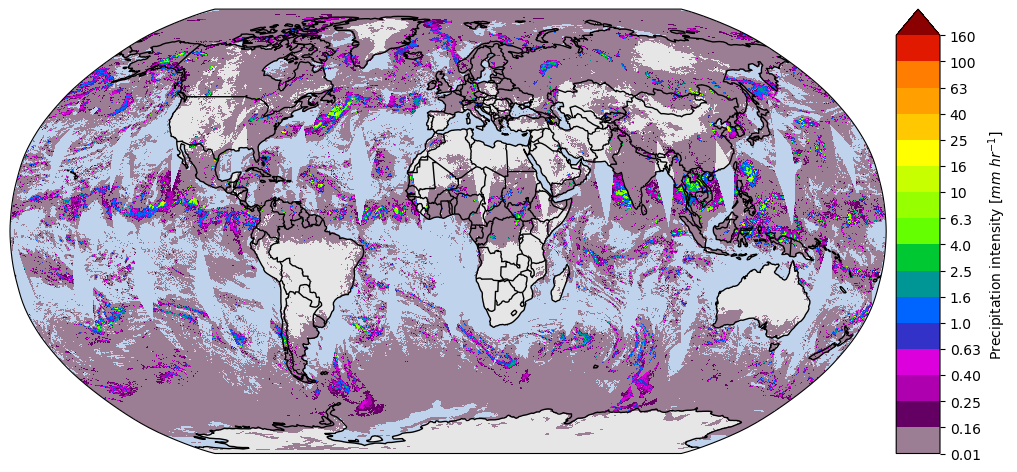
Let’s start by plotting the dataset in the geographic space:
[ ]:
da = ds[variable].isel(along_track=slice(0, 8000))
da.gpm.plot_map()
<cartopy.mpl.geocollection.GeoQuadMesh at 0x7f260777f350>

You can customize the map projection by passing a cartopy.crs.Projection to the subplot. The available projections are listed here.
[ ]:
# Define some figure options
dpi = 100
figsize = (12, 10)

# Example of Cartopy projections
crs_proj = ccrs.Robinson()  # ccrs.Orthographic(180, -90)

# Select a single variable
da = ds[variable]

# Create the map
fig, ax = plt.subplots(subplot_kw={"projection": crs_proj}, figsize=figsize, dpi=dpi)
da.gpm.plot_map(ax=ax, add_labels=False, add_background=True, add_gridlines=False, add_swath_lines=False)
ax.set_global()
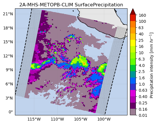
By focusing on a narrow region, it’s possible to better visualize the spatial field:
[ ]:
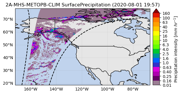
p = ds[variable].gpm.sel(gpm_id=slice(start_gpm_id, end_gpm_id)).gpm.plot_map()
p.axes.set_title(ds[variable].gpm.title(add_timestep=False))
Text(0.5, 1.0, '2A-MHS-METOPB-CLIM SurfacePrecipitation')
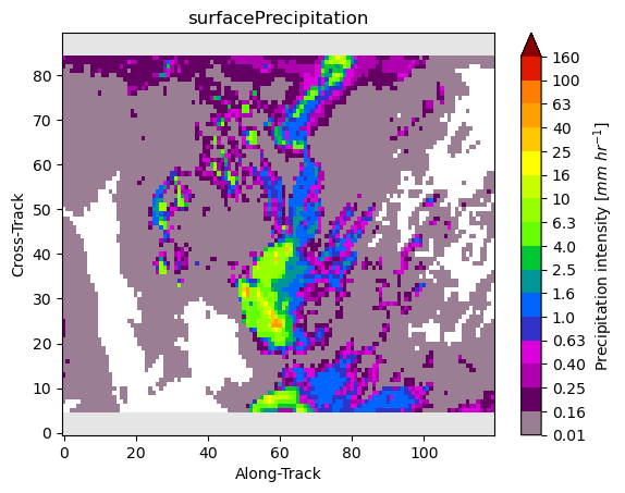
Using the gpm.plot_image method is possible to visualize the data in the so-called “swath scan view”:
[ ]:
da.gpm.plot_image()
<matplotlib.image.AxesImage at 0x7f2607496750>

[ ]:
ds[variable].gpm.sel(gpm_id=slice(start_gpm_id, end_gpm_id)).gpm.plot_image()
<matplotlib.image.AxesImage at 0x7f25fcde29d0>
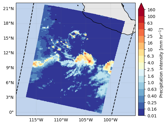
When we visualize different product variables, GPM-API will automatically try to use different appropriate colormaps and colorbars. You can observe this in the following example:
[ ]:
ds_subset = ds.gpm.sel(gpm_id=slice(start_gpm_id, end_gpm_id))
ds_subset["surfacePrecipitation"].gpm.plot_map()
ds_subset["surfacePrecipitation"].gpm.plot_map(cmap="RdYlBu_r") # ex: enable to modify defaults parameters on the fly
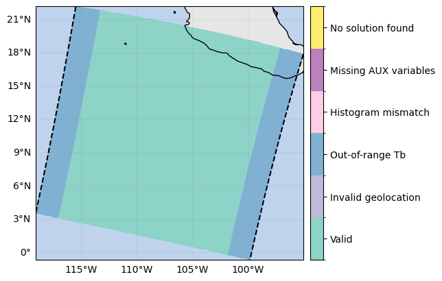
ds_subset["pixelStatus"].gpm.plot_map() # ex: defaults to categorical colorbar
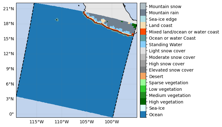
ds_subset["surfaceTypeIndex"].gpm.plot_map() # ex: defaults to categorical colorbar
<cartopy.mpl.geocollection.GeoQuadMesh at 0x7f972aec9f50>
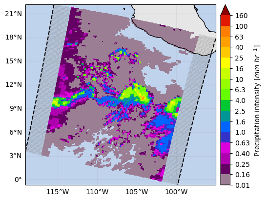
The registered colorbar configurations can be displayed using gpm.colorbars.show_colorbars() and the plot_kwargs and cbar_kwargs required to customize the figure can be obtained by calling the gpm.get_plot_kwargs function. Here below we provide an example on how to display PMW precipitation rates estimates using the same colorbar used by NASA to display IMERG liquid precipitation estimates.
GPM-API provides colormaps and colorbars tailored to GPM product variables with the goal of simplifying the data analysis and make it more reproducible.
The default colormap and colorbar configurations are defined into YAML files into the gpm/etc/colorbars directory of the software.
However, users are free to override, add and/or customize the colorbars configurations using the pycolorbar registry.
[ ]:
plot_kwargs, cbar_kwargs = gpm.get_plot_kwargs("IMERG_Liquid")
ds_subset["surfacePrecipitation"].gpm.plot_map(cbar_kwargs=cbar_kwargs, **plot_kwargs)
<cartopy.mpl.geocollection.GeoQuadMesh at 0x7f972ad84350>
5. Geospatial Manipulations#
GPM-API provides methods to easily spatially subset orbits by extent, country or continent.
Note however, that an area can be crossed by multiple orbits depending on the size of your GPM satellite dataset. In other words, multiple orbit slices in along-track direction can intersect the area of interest.
The method get_crop_slices_by_extent, get_crop_slices_by_country and get_crop_slices_by_continent enable to retrieve the orbit portions intersecting the area of interest.
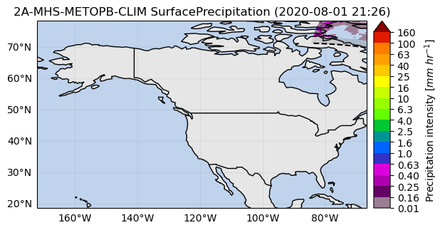
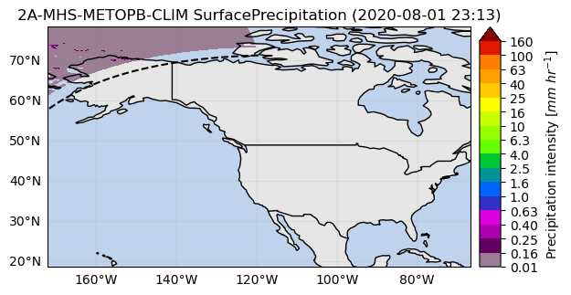
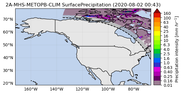
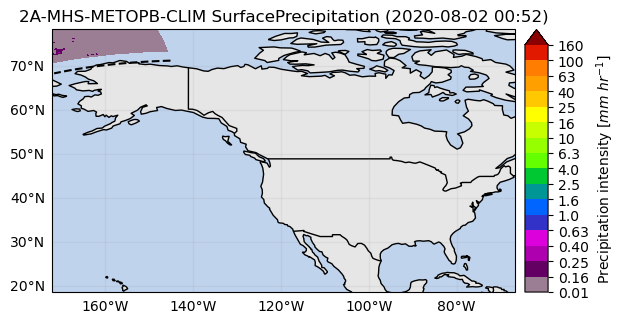
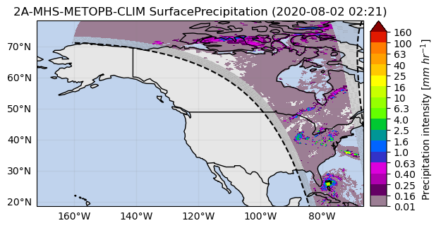
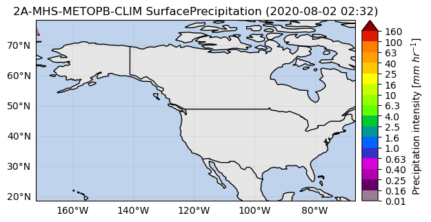
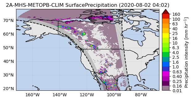
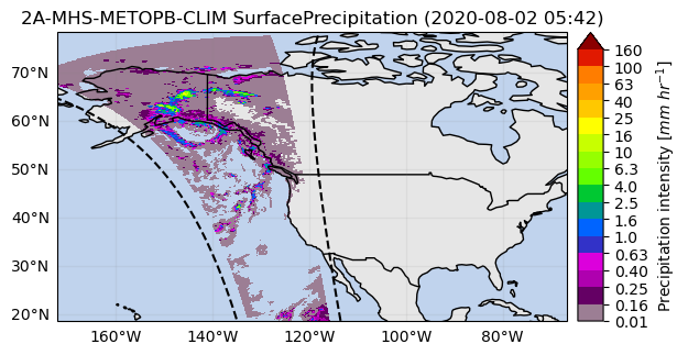
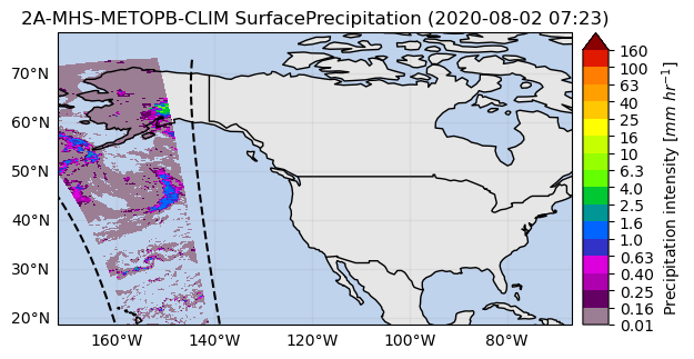
[ ]:
# Define the variable to display
variable = "surfacePrecipitation"
# Crop by country
list_isel_dict = ds.gpm.get_crop_slices_by_country("United States")
print(list_isel_dict)
# Crop by extent
extent = get_country_extent("United States")
list_isel_dict = ds.gpm.get_crop_slices_by_extent(extent)
print(list_isel_dict)
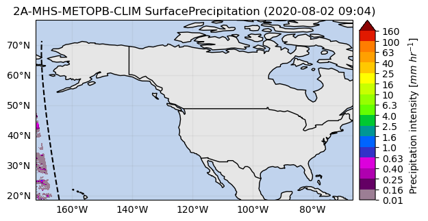
# Plot the swaths crossing the country
for isel_dict in list_isel_dict:
da_subset = ds[variable].isel(isel_dict)
slice_title = da_subset.gpm.title(add_timestep=True)
p = da_subset.gpm.plot_map()
p.axes.set_extent(extent)
p.axes.set_title(label=slice_title)
[{'along_track': slice(3772, 4119, None)}, {'along_track': slice(6030, 6400, None)}, {'along_track': slice(8273, 8680, None)}, {'along_track': slice(10509, 10961, None)}, {'along_track': slice(12733, 12770, None)}, {'along_track': slice(12790, 13216, None)}, {'along_track': slice(14940, 15051, None)}, {'along_track': slice(15070, 15225, None)}, {'along_track': slice(17041, 17332, None)}, {'along_track': slice(17351, 17410, None)}, {'along_track': slice(19163, 19612, None)}, {'along_track': slice(19631, 19635, None)}, {'along_track': slice(21439, 21865, None)}, {'along_track': slice(23720, 24103, None)}, {'along_track': slice(26001, 26354, None)}, {'along_track': slice(28281, 28623, None)}]
[{'along_track': slice(3772, 4119, None)}, {'along_track': slice(6030, 6400, None)}, {'along_track': slice(8273, 8680, None)}, {'along_track': slice(10509, 10961, None)}, {'along_track': slice(12733, 12770, None)}, {'along_track': slice(12790, 13216, None)}, {'along_track': slice(14940, 15051, None)}, {'along_track': slice(15070, 15225, None)}, {'along_track': slice(17041, 17332, None)}, {'along_track': slice(17351, 17410, None)}, {'along_track': slice(19163, 19612, None)}, {'along_track': slice(19631, 19635, None)}, {'along_track': slice(21439, 21865, None)}, {'along_track': slice(23720, 24103, None)}, {'along_track': slice(26001, 26354, None)}, {'along_track': slice(28281, 28623, None)}]
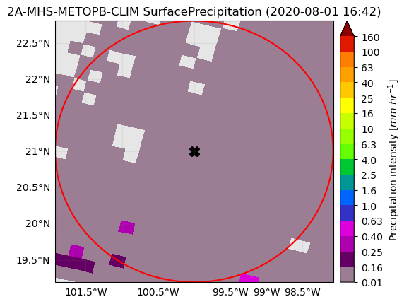
You can also easily obtain the extent around a given point (i.e. ground radar location) using the get_geographic_extent_around_point function and use the gpm accessor methods get_crop_slices_around_point or crop_around_point to subset your dataset:
[ ]:
# Define the variable to display
variable = "surfacePrecipitation"

# Crop around a point (i.e. radar location)
lon = -100
lat = 21
distance = 200_000  # 200 km
list_isel_dict = ds.gpm.get_crop_slices_around_point(
    lon=lon,
    lat=lat,
    distance=distance,
)
print(list_isel_dict)

extent = get_geographic_extent_around_point(lon=lon, lat=lat, distance=distance)
list_isel_dict = ds.gpm.get_crop_slices_by_extent(extent)
print(list_isel_dict)

# Define ROI coordinates
circle_lons, circle_lats = get_circle_coordinates_around_point(
    lon,
    lat,
    radius=distance,
    num_vertices=360,
)

# Plot the swaths crossing the ROI
for isel_dict in list_isel_dict:
    da_subset = ds[variable].isel(isel_dict)
    slice_title = da_subset.gpm.title(add_timestep=True)
    p = da_subset.gpm.plot_map()
    p.axes.set_title(slice_title)
    p.axes.plot(circle_lons, circle_lats, "r-", transform=ccrs.Geodetic())
    p.axes.scatter(lon, lat, c="black", marker="X", s=100, transform=ccrs.Geodetic())
    p.axes.set_extent(extent)
[{'along_track': slice(6353, 6380, None)}, {'along_track': slice(21454, 21481, None)}]
[{'along_track': slice(6353, 6380, None)}, {'along_track': slice(21454, 21481, None)}]

Please keep in mind that you can easily retrieve the extent of a GPM xarray object using the extent method.
The optional argument padding allows to expand/shrink the geographic extent by custom lon/lat degrees, while the size argument allows to obtain an extent centered on the GPM object with the desired size.
[ ]:
print(da_subset.gpm.extent(padding=0.1))  # expanding
print(da_subset.gpm.extent(padding=-0.1))  # shrinking
print(da_subset.gpm.extent(size=0.5))
print(da_subset.gpm.extent(size=0))  # centroid
Extent(xmin=-109.97310028076171, xmax=-88.70780029296876, ymin=16.570400619506835, ymax=25.20149955749512)
Extent(xmin=-109.77310028076172, xmax=-88.90780029296874, ymin=16.770400619506837, ymax=25.001499557495116)
Extent(xmin=-99.59045028686523, xmax=-99.09045028686523, ymin=20.635950088500977, ymax=21.135950088500977)
Extent(xmin=-99.34045028686523, xmax=-99.34045028686523, ymin=20.885950088500977, ymax=20.885950088500977)
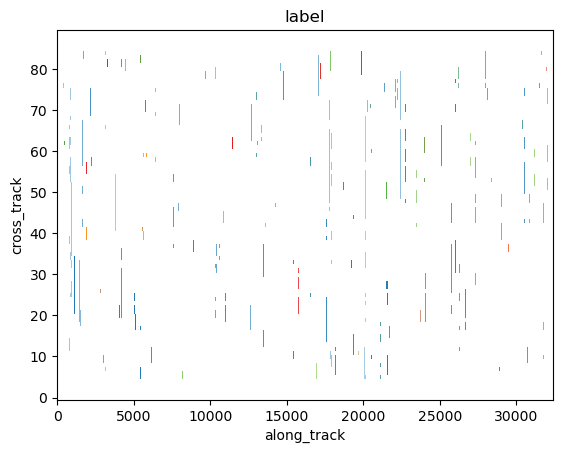
6 Storm Labeling#
Using the xarray ximage accessor, it is possible to easily delineate (label) the precipitating areas. The label array is added to the dataset as a new coordinate.
[ ]:
# Retrieve labeled xarray object
label_name = "label"
ds = ds.ximage.label(
    variable="surfacePrecipitation",
    min_value_threshold=1,
    min_area_threshold=5,
    footprint=5,  # assign same label to precipitating areas 5 pixels apart
    sort_by="area",  # "maximum", "minimum", <custom_function>
    sort_decreasing=True,
    label_name=label_name,
)
# Plot full label array
ds[label_name].ximage.plot_labels()
The array currently contains 416 labels and 'max_n_labels'
            is set to 50. The colorbar is not displayed!
<matplotlib.image.AxesImage at 0x7f974819cf90>
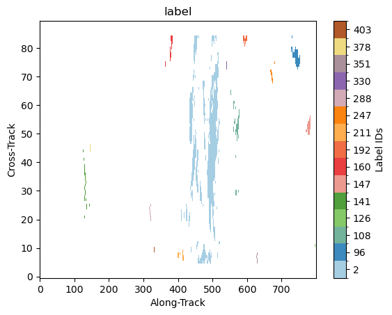
Let’s zoom in a specific region:
[ ]:
gpm.plot_labels(ds[label_name].isel(along_track=slice(2700, 3500)))
<matplotlib.image.AxesImage at 0x7f97482cd8d0>
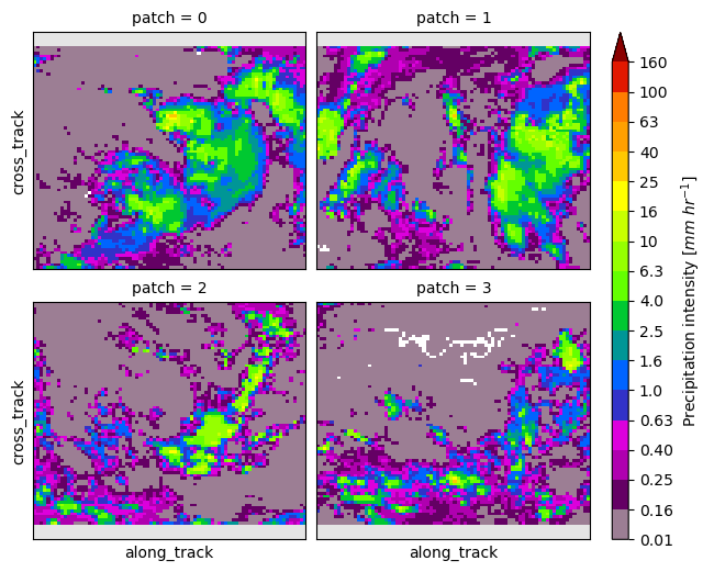
7. Patch Extraction#
With the xarray ximage accessor, it is also possible to extract patches around the precipitating areas. Here we provide a minimal example on how to proceed:
[ ]:
# Define the patch generator
da_patch_gen = ds["surfacePrecipitation"].ximage.label_patches(
    label_name=label_name,
    patch_size=(80, 80),
    # Output options
    n_patches=4,
    # Patch extraction Options
    padding=0,
    centered_on="max",
    # Tiling/Sliding Options
    debug=False,
    verbose=False,
)

# # Retrieve list of patches
list_label_patches = list(da_patch_gen)
list_da = [da for label, da in list_label_patches]

# Display patches
gpm.plot_patches(list_label_patches)

You can exploit the xarray manipulations and FacetGrid capabilities to quickly create the following figure:
[ ]:
list_da_without_coords = [da.drop_vars(["lon", "lat"]) for da in list_da]
da_patch = xr.concat(list_da_without_coords, dim="patch")
da_patch.isel(patch=slice(0, 4)).gpm.plot_image(col="patch", col_wrap=2)
<gpm.visualization.facetgrid.ImageFacetGrid at 0x7f972ace6ad0>