PMW 1B and 1C products#
In this tutorial, we will provide the foundations to use GPM-API to download, manipulate and analyze data from the Global Precipitation Measurement (GPM) Passive Microwave (PMW) 1B and 1C products.
Please note that GPM-API also enable access and analysis tools for the entire GPM constellation of passive microwave sensors as well as the IMERG precipitation products. For detailed information and additional tutorials, please refer to the others GPM-API tutorials.
First, let’s import the package required in this tutorial.
[ ]:
import datetime

import cartopy.crs as ccrs
import matplotlib.pyplot as plt
import xarray as xr
import ximage  # noqa

import gpm
from gpm.utils.geospatial import (
    get_circle_coordinates_around_point,
    get_continent_extent,
    get_country_extent,
    get_geographic_extent_around_point,
)
Let’s have a look at the available PMW Level 1 products:
[ ]:
gpm.available_products(product_categories="PMW", product_levels="1B")
['1B-GMI', '1B-TMI']
[ ]:
gpm.available_products(product_categories="PMW", product_levels="1C")
['1C-AMSR2-GCOMW1',
 '1C-AMSRE-AQUA',
 '1C-AMSUB-NOAA15',
 '1C-AMSUB-NOAA16',
 '1C-AMSUB-NOAA17',
 '1C-ATMS-NOAA20',
 '1C-ATMS-NOAA21',
 '1C-ATMS-NPP',
 '1C-GMI',
 '1C-GMI-R',
 '1C-MHS-METOPA',
 '1C-MHS-METOPB',
 '1C-MHS-METOPC',
 '1C-MHS-NOAA18',
 '1C-MHS-NOAA19',
 '1C-SAPHIR-MT1',
 '1C-SSMI-F08',
 '1C-SSMI-F10',
 '1C-SSMI-F11',
 '1C-SSMI-F13',
 '1C-SSMI-F14',
 '1C-SSMI-F15',
 '1C-SSMIS-F16',
 '1C-SSMIS-F17',
 '1C-SSMIS-F18',
 '1C-SSMIS-F19',
 '1C-TMI']
The GPM Level 1B products provides the “raw” brightness temperature (BTs) measured from the GPM Microwave Imager (GMI) and TRMM Microwave Imager (TMI) sensors. In contrast, the GPM Level 1C products provides a intercalibrated BTs dataset for each microwave radiometer in the GPM constellation, using GMI and TMI as the calibration reference.
Each L1B and L1C data file, referred as an orbital granule, spans exactly one orbit, starting and ending at the satellite’s southernmost latitude. The L1C products also provides comprehensive per-footprint and per-scan quality flags, highlighting potential issues such as missing scans, invalid geolocation, sun glint, or radio-frequency interference (RFI).
The PMW sensor channels are grouped into scan modes (e.g. S1, S2) based on their native scan geometry (i.e. different viewing geometries). Because these scan modes are not spatially collocated, you will often need to remap them onto a common grid for joint analysis.
To this end, in this tutoria we will also illustrate how to use GPM-API to remap all channels to a single grid. Note that the 1C-GMI-R product is already a remapped version of 1C-GMI, where the higher-frequency S2 channels have been nearest-neighbor mapped onto the S1 geometry.
For additional details, please consult the L1C PMW Products ATBD.
1. Download Data#
Now let’s download a 1C PMW product over a couple of hours.
To download GPM data with GPM-API, you have to previously create a NASA Earthdata and/or NASA PPS account. We provide a step-by-step guide on how to set up your accounts in the official GPM-API documentation.
[ ]:
# Specify the time period you are interested in
start_time = datetime.datetime.strptime("2021-08-29 10:00:00", "%Y-%m-%d %H:%M:%S")
end_time = datetime.datetime.strptime("2021-08-29 16:00:00", "%Y-%m-%d %H:%M:%S")
# Specify the product and product type
product = "1C-SSMIS-F18"  # 1C-GMI, ...
product_type = "RS"
storage = "PPS"
# Specify the version
version = 7
[ ]:
# Download the data
gpm.download(
    product=product,
    product_type=product_type,
    version=version,
    start_time=start_time,
    end_time=end_time,
    storage=storage,
    force_download=False,
    verbose=True,
    progress_bar=True,
    check_integrity=False,
)
All the available GPM 1C-SSMIS-F18 product files are already on disk.
Once, the data are downloaded on disk, let’s load the 1C product and look at the dataset structure.
2. Load Data#
With GPM-API, the name granule is used to refer to a single file, while the name dataset is used to refer to a collection of granules.
GPM-API enables to open single or multiple granules into xarray, a software designed for working with labeled multi-dimensional arrays.
The
gpm.open_granule_dataset(filepath)opens a singlescan_modeof a granule into axarray.Datasetobject by providing the path of the file of interest.The
gpm.open_granule_datatree(filepath)opens allscan_modesof granule into axarray.DataTreeobject by providing the path of the file of interest.The
gpm.open_datasetandgpm.open_datatreefunctions enable to open a collection of granules over a period of interest intoxarray.Datasetandxarray.DataTreeobjects respectively.
Before loading a product, one can already list the available scan modes with:
[ ]:
gpm.available_scan_modes(product=product, version=version)
['S1', 'S2', 'S3', 'S4']
Now let’s open the 1C PMW product with gpm_open_datatree and look at the dataset structure.
[ ]:
dt = gpm.open_datatree(
    product=product,
    product_type=product_type,
    version=version,
    start_time=start_time,
    end_time=end_time,
)
print("Available scan modes:", list(dt))
dt
Available scan modes: ['S1', 'S2', 'S3', 'S4']
<xarray.DatasetView> Size: 0B
Dimensions:  ()
Data variables:
*empty*A single scan mode dataset can be extracted from the DataTree object using:
[ ]:
ds_s1 = dt["S1"].to_dataset()
ds_s1
<xarray.Dataset> Size: 54MB
Dimensions:                  (cross_track: 90, along_track: 11377,
                              pmw_frequency: 3)
Coordinates:
    sunLocalTime             (cross_track, along_track) float32 4MB dask.array<chunksize=(90, 1660), meta=np.ndarray>
    Quality                  (cross_track, along_track) float32 4MB dask.array<chunksize=(90, 1660), meta=np.ndarray>
    SCorientation            (along_track) float32 46kB dask.array<chunksize=(1660,), meta=np.ndarray>
    lon                      (cross_track, along_track) float32 4MB 87.31 ......
    lat                      (cross_track, along_track) float32 4MB 86.83 ......
    time                     (along_track) datetime64[ns] 91kB 2021-08-29T10:...
    gpm_id                   (along_track) <U10 455kB ...
    gpm_granule_id           (along_track) int64 91kB ...
    gpm_cross_track_id       (cross_track) int64 720B ...
    gpm_along_track_id       (along_track) int64 91kB ...
  * pmw_frequency            (pmw_frequency) <U3 36B '19V' '19H' '22V'
    crsWGS84                 int64 8B 0
Dimensions without coordinates: cross_track, along_track
Data variables:
    incidenceAngle           (cross_track, along_track, pmw_frequency) float32 12MB dask.array<chunksize=(90, 11377, 3), meta=np.ndarray>
    sunGlintAngle            (cross_track, along_track, pmw_frequency) float32 12MB dask.array<chunksize=(90, 11377, 3), meta=np.ndarray>
    Tc                       (cross_track, along_track, pmw_frequency) float32 12MB dask.array<chunksize=(90, 1660, 3), meta=np.ndarray>
    SClatitude               (along_track) float32 46kB dask.array<chunksize=(1660,), meta=np.ndarray>
    SClongitude              (along_track) float32 46kB dask.array<chunksize=(1660,), meta=np.ndarray>
    SCaltitude               (along_track) float32 46kB dask.array<chunksize=(1660,), meta=np.ndarray>
    FractionalGranuleNumber  (along_track) float64 91kB dask.array<chunksize=(1660,), meta=np.ndarray>
Attributes: (12/17)
    FileName:           1C.F18.SSMIS.XCAL2021-V.20210829-S091036-E105231.0611...
    EphemerisFileName:
    AttitudeFileName:
    MissingData:        0
    DOI:                10.5067/GPM/SSMIS/F18/1C/07
    DOIauthority:       http://dx.doi.org/
    ...                 ...
    ProcessingSystem:   PPS
    DataFormatVersion:  7e
    MetadataVersion:    7e
    ScanMode:           S1
    history:            Created by ghiggi/gpm_api software on 2025-03-05 20:4...
gpm_api_product: 1C-SSMIS-F18If you need to analyze a specific scan mode, is more efficient to just read in directly that scan mode using gpm.open_dataset:
[ ]:
ds_s1 = gpm.open_dataset(
    product=product,
    product_type=product_type,
    version=version,
    start_time=start_time,
    end_time=end_time,
    scan_mode="S1",
)
ds_s1
<xarray.Dataset> Size: 54MB
Dimensions:                  (cross_track: 90, along_track: 11377,
                              pmw_frequency: 3)
Coordinates:
    sunLocalTime             (cross_track, along_track) float32 4MB dask.array<chunksize=(90, 1660), meta=np.ndarray>
    Quality                  (cross_track, along_track) float32 4MB dask.array<chunksize=(90, 1660), meta=np.ndarray>
    SCorientation            (along_track) float32 46kB dask.array<chunksize=(1660,), meta=np.ndarray>
    lon                      (cross_track, along_track) float32 4MB 87.31 ......
    lat                      (cross_track, along_track) float32 4MB 86.83 ......
    time                     (along_track) datetime64[ns] 91kB 2021-08-29T10:...
    gpm_id                   (along_track) <U10 455kB ...
    gpm_granule_id           (along_track) int64 91kB ...
    gpm_cross_track_id       (cross_track) int64 720B ...
    gpm_along_track_id       (along_track) int64 91kB ...
  * pmw_frequency            (pmw_frequency) <U3 36B '19V' '19H' '22V'
    crsWGS84                 int64 8B 0
Dimensions without coordinates: cross_track, along_track
Data variables:
    incidenceAngle           (cross_track, along_track, pmw_frequency) float32 12MB dask.array<chunksize=(90, 11377, 3), meta=np.ndarray>
    sunGlintAngle            (cross_track, along_track, pmw_frequency) float32 12MB dask.array<chunksize=(90, 11377, 3), meta=np.ndarray>
    Tc                       (cross_track, along_track, pmw_frequency) float32 12MB dask.array<chunksize=(90, 1660, 3), meta=np.ndarray>
    SClatitude               (along_track) float32 46kB dask.array<chunksize=(1660,), meta=np.ndarray>
    SClongitude              (along_track) float32 46kB dask.array<chunksize=(1660,), meta=np.ndarray>
    SCaltitude               (along_track) float32 46kB dask.array<chunksize=(1660,), meta=np.ndarray>
    FractionalGranuleNumber  (along_track) float64 91kB dask.array<chunksize=(1660,), meta=np.ndarray>
Attributes: (12/17)
    FileName:           1C.F18.SSMIS.XCAL2021-V.20210829-S091036-E105231.0611...
    EphemerisFileName:
    AttitudeFileName:
    MissingData:        0
    DOI:                10.5067/GPM/SSMIS/F18/1C/07
    DOIauthority:       http://dx.doi.org/
    ...                 ...
    ProcessingSystem:   PPS
    DataFormatVersion:  7e
    MetadataVersion:    7e
    ScanMode:           S1
    history:            Created by ghiggi/gpm_api software on 2025-03-05 20:4...
gpm_api_product: 1C-SSMIS-F183. Remapping Data#
As we introduced before, PMW channel across scan modes are not spatially collocated.
Here below we nearest-neighbour remap all scan modes to a unique reference grid.
Please remember that remapping all scan modes to the first ‘S1’ scan mode means downsampling high-frequency channels. Reversely, remapping all scan modes to higher scan modes (the ones containing high-frequency channels), means oversampling low-frequency channels but obtaining higher resolution grid.
[ ]:
ds = dt.gpm.regrid_pmw_l1(scan_mode_reference="S1")  # this might take a moment
ds
<xarray.Dataset> Size: 177MB
Dimensions:             (cross_track: 90, along_track: 11377,
                         pmw_frequency: 11, scan_mode: 4)
Coordinates:
    SCorientation       (along_track) float32 46kB dask.array<chunksize=(886,), meta=np.ndarray>
    lon                 (cross_track, along_track) float32 4MB 87.31 ... 9.236
    lat                 (cross_track, along_track) float32 4MB 86.83 ... -81.26
    time                (along_track) datetime64[ns] 91kB 2021-08-29T10:00:00...
    gpm_id              (along_track) <U10 455kB '61187-1561' ... '61191-51'
    gpm_granule_id      (along_track) int64 91kB 61187 61187 ... 61191 61191
    gpm_cross_track_id  (cross_track) int64 720B ...
    gpm_along_track_id  (along_track) int64 91kB 1561 1562 1563 ... 49 50 51
  * pmw_frequency       (pmw_frequency) <U5 220B '19V' '19H' ... '91V' '91H'
    crsWGS84            int64 8B 0
  * scan_mode           (scan_mode) <U2 32B 'S1' 'S2' 'S3' 'S4'
Dimensions without coordinates: cross_track, along_track
Data variables:
    incidenceAngle      (cross_track, along_track, pmw_frequency) float32 45MB dask.array<chunksize=(90, 886, 3), meta=np.ndarray>
    sunGlintAngle       (cross_track, along_track, pmw_frequency) float32 45MB dask.array<chunksize=(90, 886, 3), meta=np.ndarray>
    Tc                  (cross_track, along_track, pmw_frequency) float32 45MB dask.array<chunksize=(90, 886, 3), meta=np.ndarray>
    sunLocalTime        (cross_track, along_track, scan_mode) float32 16MB dask.array<chunksize=(90, 886, 1), meta=np.ndarray>
    Quality             (cross_track, along_track, scan_mode) float32 16MB dask.array<chunksize=(90, 886, 1), meta=np.ndarray>
Attributes: (12/18)
    FileName:           1C.F18.SSMIS.XCAL2021-V.20210829-S091036-E105231.0611...
    EphemerisFileName:
    AttitudeFileName:
    MissingData:        0
    DOI:                10.5067/GPM/SSMIS/F18/1C/07
    DOIauthority:       http://dx.doi.org/
    ...                 ...
    DataFormatVersion:  7e
    MetadataVersion:    7e
    ScanMode:           S1
    history:            Created by ghiggi/gpm_api software on 2025-03-05 20:4...
    gpm_api_product:    1C-SSMIS-F18
ScanModes: ['S1', 'S2', 'S3', 'S4']4. Basic Manipulations#
Once you have a xarray.Dataset, you can list variables, coordinates and dimensions with the following methods
[ ]:
# Available variables
variables = list(ds.data_vars)
print("Available variables: ", variables)
# Available coordinates
coords = list(ds.coords)
print("Available coordinates: ", coords)
# Available dimensions
dims = list(ds.dims)
print("Available dimensions: ", dims)
Available variables: ['incidenceAngle', 'sunGlintAngle', 'Tc', 'sunLocalTime', 'Quality']
Available coordinates: ['SCorientation', 'lon', 'lat', 'time', 'gpm_id', 'gpm_granule_id', 'gpm_cross_track_id', 'gpm_along_track_id', 'pmw_frequency', 'crsWGS84', 'scan_mode']
Available dimensions: ['cross_track', 'along_track', 'pmw_frequency', 'scan_mode']
To select the DataArray corresponding to a single variable:
[ ]:
variable = "Tc" # "Tb" if PMW 1B product
da = ds[variable]
print("Array class: ", type(da.data))
da
Array class: <class 'dask.array.core.Array'>
<xarray.DataArray 'Tc' (cross_track: 90, along_track: 11377, pmw_frequency: 11)> Size: 45MB
dask.array<concatenate, shape=(90, 11377, 11), dtype=float32, chunksize=(90, 886, 4), chunktype=numpy.ndarray>
Coordinates:
SCorientation (along_track) float32 46kB dask.array<chunksize=(886,), meta=np.ndarray>
lon (cross_track, along_track) float32 4MB 87.31 ... 9.236
lat (cross_track, along_track) float32 4MB 86.83 ... -81.26
time (along_track) datetime64[ns] 91kB 2021-08-29T10:00:00...
gpm_id (along_track) <U10 455kB '61187-1561' ... '61191-51'
gpm_granule_id (along_track) int64 91kB 61187 61187 ... 61191 61191
gpm_cross_track_id (cross_track) int64 720B ...
gpm_along_track_id (along_track) int64 91kB 1561 1562 1563 ... 49 50 51
* pmw_frequency (pmw_frequency) <U5 220B '19V' '19H' ... '91V' '91H'
crsWGS84 int64 8B 0
Dimensions without coordinates: cross_track, along_track
Attributes:
units: K
description: Intercalibrated Tb for channels 1) 19.35 GHz V-Pol 2) 1...
gpm_api_product: 1C-SSMIS-F18
grid_mapping: crsWGS84If the array class is dask.Array, it means that the data are not yet loaded into RAM memory. To put the data into memory, you need to call the method compute, either on the xarray object or on the numerical array.
[ ]:
da = da.compute()
print("Array class: ", type(da.data))
da
Array class: <class 'numpy.ndarray'>
<xarray.DataArray 'Tc' (cross_track: 90, along_track: 11377, pmw_frequency: 11)> Size: 45MB
array([[[228.58, 200.79, 227.83, ..., 259.74, 223.95, 214.76],
[228.7 , 200.33, 227.64, ..., 260.53, 222.65, 215.09],
[228.92, 199.33, 227.76, ..., 254.1 , 226.07, 217.92],
...,
[176.48, 147.97, 184.55, ..., nan, 219.03, 201.14],
[182.93, 155.26, 190.26, ..., nan, 223.62, 203.41],
[190.51, 164.68, 197.11, ..., nan, 222.5 , 201.11]],
[[229.74, 199.74, 228.22, ..., 254.1 , 226.07, 217.92],
[229.77, 199.46, 228.62, ..., 256.19, 229.02, 221.4 ],
[228.61, 198.07, 227.65, ..., 258.71, 224.07, 217.31],
...,
[192.97, 167.43, 199.03, ..., 238.56, 222.5 , 201.11],
[200.62, 176.02, 205.22, ..., 238.88, 226.57, 202.67],
[206.74, 183.1 , 210.44, ..., nan, 228.95, 205.98]],
[[228.98, 198.76, 227.53, ..., 258.71, 221.11, 211.9 ],
[228.7 , 196.76, 227.21, ..., 255.67, 221.71, 212.41],
[228.06, 195.71, 225.75, ..., 257.5 , 221.46, 211.99],
...,
...
[166.61, 122.73, 164.86, ..., 162.27, 164.05, 142.47],
[163.75, 120.81, 162.6 , ..., 154.9 , 160.82, 139.2 ],
[164.24, 121.18, 162.62, ..., 148.96, 159.99, 139.13]],
[[193.91, 131.26, 215.64, ..., 268.18, 264.74, 249.33],
[192.92, 129.03, 214.26, ..., 270.79, 262.64, 244.24],
[192.53, 127.28, 212.9 , ..., 268.07, 259.68, 236.52],
...,
[177.88, 129.69, 175.91, ..., 167.58, 174.39, 151.56],
[173.17, 126.34, 171.33, ..., 157.68, 176.14, 155.03],
[167.81, 123.5 , 166.4 , ..., 164.5 , 163.73, 142.15]],
[[194.04, 131.81, 216.79, ..., 262.46, 267.03, 255.5 ],
[194.02, 132.13, 216.97, ..., 268.45, 267.59, 256.87],
[193.63, 130.63, 215.6 , ..., 268.18, 265.16, 251.8 ],
...,
[185.3 , 135.13, 182.51, ..., 168.67, 175.06, 153.83],
[182.57, 133. , 179.64, ..., 164.51, 177.62, 156.23],
[179.62, 130.88, 177.91, ..., 167.58, 174.39, 151.56]]],
dtype=float32)
Coordinates:
SCorientation (along_track) float32 46kB 0.0 0.0 0.0 ... 0.0 0.0 0.0
lon (cross_track, along_track) float32 4MB 87.31 ... 9.236
lat (cross_track, along_track) float32 4MB 86.83 ... -81.26
time (along_track) datetime64[ns] 91kB 2021-08-29T10:00:00...
gpm_id (along_track) <U10 455kB '61187-1561' ... '61191-51'
gpm_granule_id (along_track) int64 91kB 61187 61187 ... 61191 61191
gpm_cross_track_id (cross_track) int64 720B 0 1 2 3 4 5 ... 85 86 87 88 89
gpm_along_track_id (along_track) int64 91kB 1561 1562 1563 ... 49 50 51
* pmw_frequency (pmw_frequency) <U5 220B '19V' '19H' ... '91V' '91H'
crsWGS84 int64 8B 0
Dimensions without coordinates: cross_track, along_track
Attributes:
units: K
description: Intercalibrated Tb for channels 1) 19.35 GHz V-Pol 2) 1...
gpm_api_product: 1C-SSMIS-F18
grid_mapping: crsWGS84To extract the array from the xarray.DataArray, you can use:
[ ]:
da.data
array([[[228.58, 200.79, 227.83, ..., 259.74, 223.95, 214.76],
[228.7 , 200.33, 227.64, ..., 260.53, 222.65, 215.09],
[228.92, 199.33, 227.76, ..., 254.1 , 226.07, 217.92],
...,
[176.48, 147.97, 184.55, ..., nan, 219.03, 201.14],
[182.93, 155.26, 190.26, ..., nan, 223.62, 203.41],
[190.51, 164.68, 197.11, ..., nan, 222.5 , 201.11]],
[[229.74, 199.74, 228.22, ..., 254.1 , 226.07, 217.92],
[229.77, 199.46, 228.62, ..., 256.19, 229.02, 221.4 ],
[228.61, 198.07, 227.65, ..., 258.71, 224.07, 217.31],
...,
[192.97, 167.43, 199.03, ..., 238.56, 222.5 , 201.11],
[200.62, 176.02, 205.22, ..., 238.88, 226.57, 202.67],
[206.74, 183.1 , 210.44, ..., nan, 228.95, 205.98]],
[[228.98, 198.76, 227.53, ..., 258.71, 221.11, 211.9 ],
[228.7 , 196.76, 227.21, ..., 255.67, 221.71, 212.41],
[228.06, 195.71, 225.75, ..., 257.5 , 221.46, 211.99],
...,
[209.25, 186.17, 212.79, ..., 239.84, 228.95, 205.98],
[213.2 , 190.93, 215.35, ..., 235.76, 229.9 , 206.97],
[216.3 , 193.41, 217.79, ..., nan, 224.35, 205.34]],
...,
[[191.85, 127.79, 213.34, ..., 268.97, 262.52, 244.93],
[191.02, 125.89, 211.96, ..., 266.09, 261.54, 241.87],
[190.2 , 124.15, 210.59, ..., 271.81, 259.05, 233.51],
...,
[166.61, 122.73, 164.86, ..., 162.27, 164.05, 142.47],
[163.75, 120.81, 162.6 , ..., 154.9 , 160.82, 139.2 ],
[164.24, 121.18, 162.62, ..., 148.96, 159.99, 139.13]],
[[193.91, 131.26, 215.64, ..., 268.18, 264.74, 249.33],
[192.92, 129.03, 214.26, ..., 270.79, 262.64, 244.24],
[192.53, 127.28, 212.9 , ..., 268.07, 259.68, 236.52],
...,
[177.88, 129.69, 175.91, ..., 167.58, 174.39, 151.56],
[173.17, 126.34, 171.33, ..., 157.68, 176.14, 155.03],
[167.81, 123.5 , 166.4 , ..., 164.5 , 163.73, 142.15]],
[[194.04, 131.81, 216.79, ..., 262.46, 267.03, 255.5 ],
[194.02, 132.13, 216.97, ..., 268.45, 267.59, 256.87],
[193.63, 130.63, 215.6 , ..., 268.18, 265.16, 251.8 ],
...,
[185.3 , 135.13, 182.51, ..., 168.67, 175.06, 153.83],
[182.57, 133. , 179.64, ..., 164.51, 177.62, 156.23],
[179.62, 130.88, 177.91, ..., 167.58, 174.39, 151.56]]],
dtype=float32)
The list of dataset variables which have a pmw_frequency dimension can be obtained with:
[ ]:
ds.gpm.frequency_variables
['Tc', 'incidenceAngle', 'sunGlintAngle']
The list of PMW channels can be obtained using:
[ ]:
ds["pmw_frequency"]
<xarray.DataArray 'pmw_frequency' (pmw_frequency: 11)> Size: 220B
array(['19V', '19H', '22V', '37V', '37H', '150H', '183H1', '183H3', '183H7',
       '91V', '91H'], dtype='<U5')
Coordinates:
* pmw_frequency (pmw_frequency) <U5 220B '19V' '19H' '22V' ... '91V' '91H'
crsWGS84 int64 8B 0You can subset the dataset along the pmw_frequency dimension by indexing (with isel) or by value (with sel):
[ ]:
ds.isel(pmw_frequency=0)
ds.sel(pmw_frequency="19V")
<xarray.Dataset> Size: 54MB
Dimensions:             (cross_track: 90, along_track: 11377, scan_mode: 4)
Coordinates:
    SCorientation       (along_track) float32 46kB dask.array<chunksize=(886,), meta=np.ndarray>
    lon                 (cross_track, along_track) float32 4MB 87.31 ... 9.236
    lat                 (cross_track, along_track) float32 4MB 86.83 ... -81.26
    time                (along_track) datetime64[ns] 91kB 2021-08-29T10:00:00...
    gpm_id              (along_track) <U10 455kB '61187-1561' ... '61191-51'
    gpm_granule_id      (along_track) int64 91kB 61187 61187 ... 61191 61191
    gpm_cross_track_id  (cross_track) int64 720B ...
    gpm_along_track_id  (along_track) int64 91kB 1561 1562 1563 ... 49 50 51
    pmw_frequency       <U5 20B '19V'
    crsWGS84            int64 8B 0
  * scan_mode           (scan_mode) <U2 32B 'S1' 'S2' 'S3' 'S4'
Dimensions without coordinates: cross_track, along_track
Data variables:
    incidenceAngle      (cross_track, along_track) float32 4MB dask.array<chunksize=(90, 886), meta=np.ndarray>
    sunGlintAngle       (cross_track, along_track) float32 4MB dask.array<chunksize=(90, 886), meta=np.ndarray>
    Tc                  (cross_track, along_track) float32 4MB dask.array<chunksize=(90, 886), meta=np.ndarray>
    sunLocalTime        (cross_track, along_track, scan_mode) float32 16MB dask.array<chunksize=(90, 886, 1), meta=np.ndarray>
    Quality             (cross_track, along_track, scan_mode) float32 16MB dask.array<chunksize=(90, 886, 1), meta=np.ndarray>
Attributes: (12/18)
    FileName:           1C.F18.SSMIS.XCAL2021-V.20210829-S091036-E105231.0611...
    EphemerisFileName:
    AttitudeFileName:
    MissingData:        0
    DOI:                10.5067/GPM/SSMIS/F18/1C/07
    DOIauthority:       http://dx.doi.org/
    ...                 ...
    DataFormatVersion:  7e
    MetadataVersion:    7e
    ScanMode:           S1
    history:            Created by ghiggi/gpm_api software on 2025-03-05 20:4...
    gpm_api_product:    1C-SSMIS-F18
ScanModes: ['S1', 'S2', 'S3', 'S4']Since xarray does not yet allow subsetting by value along non-dimensional coordinates, the gpm.sel method provides you this functionality.
As an example, you can subset the dataset by time:
[ ]:
start_time = datetime.datetime.strptime("2021-08-29 10:00:00", "%Y-%m-%d %H:%M:%S")
end_time = datetime.datetime.strptime("2021-08-29 10:30:00", "%Y-%m-%d %H:%M:%S")
ds_subset = ds.gpm.sel(time=slice(start_time, end_time))
ds_subset["time"]
<xarray.DataArray 'time' (along_track: 949)> Size: 8kB
array(['2021-08-29T10:00:00.000000000', '2021-08-29T10:00:02.000000000',
       '2021-08-29T10:00:04.000000000', '2021-08-29T10:00:06.000000000',
       '2021-08-29T10:00:08.000000000', '2021-08-29T10:00:10.000000000',
       '2021-08-29T10:00:12.000000000', '2021-08-29T10:00:13.000000000',
       '2021-08-29T10:00:15.000000000', '2021-08-29T10:00:17.000000000',
       '2021-08-29T10:00:19.000000000', '2021-08-29T10:00:21.000000000',
       '2021-08-29T10:00:23.000000000', '2021-08-29T10:00:25.000000000',
       '2021-08-29T10:00:27.000000000', '2021-08-29T10:00:29.000000000',
       '2021-08-29T10:00:31.000000000', '2021-08-29T10:00:32.000000000',
       '2021-08-29T10:00:34.000000000', '2021-08-29T10:00:36.000000000',
       '2021-08-29T10:00:38.000000000', '2021-08-29T10:00:40.000000000',
       '2021-08-29T10:00:42.000000000', '2021-08-29T10:00:44.000000000',
       '2021-08-29T10:00:46.000000000', '2021-08-29T10:00:48.000000000',
       '2021-08-29T10:00:50.000000000', '2021-08-29T10:00:51.000000000',
       '2021-08-29T10:00:53.000000000', '2021-08-29T10:00:55.000000000',
       '2021-08-29T10:00:57.000000000', '2021-08-29T10:00:59.000000000',
       '2021-08-29T10:01:01.000000000', '2021-08-29T10:01:03.000000000',
       '2021-08-29T10:01:05.000000000', '2021-08-29T10:01:07.000000000',
       '2021-08-29T10:01:08.000000000', '2021-08-29T10:01:10.000000000',
       '2021-08-29T10:01:12.000000000', '2021-08-29T10:01:14.000000000',
...
       '2021-08-29T10:28:48.000000000', '2021-08-29T10:28:50.000000000',
       '2021-08-29T10:28:52.000000000', '2021-08-29T10:28:54.000000000',
       '2021-08-29T10:28:56.000000000', '2021-08-29T10:28:57.000000000',
       '2021-08-29T10:28:59.000000000', '2021-08-29T10:29:01.000000000',
       '2021-08-29T10:29:03.000000000', '2021-08-29T10:29:05.000000000',
       '2021-08-29T10:29:07.000000000', '2021-08-29T10:29:09.000000000',
       '2021-08-29T10:29:11.000000000', '2021-08-29T10:29:13.000000000',
       '2021-08-29T10:29:15.000000000', '2021-08-29T10:29:16.000000000',
       '2021-08-29T10:29:18.000000000', '2021-08-29T10:29:20.000000000',
       '2021-08-29T10:29:22.000000000', '2021-08-29T10:29:24.000000000',
       '2021-08-29T10:29:26.000000000', '2021-08-29T10:29:28.000000000',
       '2021-08-29T10:29:30.000000000', '2021-08-29T10:29:32.000000000',
       '2021-08-29T10:29:34.000000000', '2021-08-29T10:29:35.000000000',
       '2021-08-29T10:29:37.000000000', '2021-08-29T10:29:39.000000000',
       '2021-08-29T10:29:41.000000000', '2021-08-29T10:29:43.000000000',
       '2021-08-29T10:29:45.000000000', '2021-08-29T10:29:47.000000000',
       '2021-08-29T10:29:49.000000000', '2021-08-29T10:29:51.000000000',
       '2021-08-29T10:29:53.000000000', '2021-08-29T10:29:54.000000000',
       '2021-08-29T10:29:56.000000000', '2021-08-29T10:29:58.000000000',
       '2021-08-29T10:30:00.000000000'], dtype='datetime64[ns]')
Coordinates:
    SCorientation       (along_track) float32 4kB dask.array<chunksize=(886,), meta=np.ndarray>
    time                (along_track) datetime64[ns] 8kB 2021-08-29T10:00:00 ...
    gpm_id              (along_track) <U10 38kB '61187-1561' ... '61187-2509'
    gpm_granule_id      (along_track) int64 8kB 61187 61187 ... 61187 61187
    gpm_along_track_id  (along_track) int64 8kB 1561 1562 1563 ... 2508 2509
    crsWGS84            int64 8B 0
Dimensions without coordinates: along_track
Attributes:
    standard_name:          time
    coverage_content_type:  coordinate
axis: TRemember that you can get the start time and end time of your GPM xarray object with the gpm accessor methods start_time and end_time.
[ ]:
print(ds_subset.gpm.start_time)
print(ds_subset.gpm.end_time)
2021-08-29 10:00:00
2021-08-29 10:30:00
You can also subset your GPM xarray object by gpm_id and gpm_cross_track_id` coordinates, which act as reference identifiers for the along-track, cross-track dimensions. Selecting across coordinates by value is useful for example to: - align multiple GPM xarray objects that might have been subsetted differently across the`cross_track,along_track` dimensions. - to retrieve a specific portion of a GPM granule indipendently of the previous subsetting operations.
The gpm_id is defined as <gpm_granule_number>-<gpm_along_track_id>, while the others <gpm_*_id> coordinates start at 0 and increase incrementally by 1 along each granule dimension.
[ ]:
# Subset by gpm_id
start_gpm_id = "61187-2000"
end_gpm_id = "61187-2200"
ds_subset = ds.gpm.sel(gpm_id=slice(start_gpm_id, end_gpm_id))
ds_subset["gpm_id"].data
array(['61187-2000', '61187-2001', '61187-2002', '61187-2003',
       '61187-2004', '61187-2005', '61187-2006', '61187-2007',
       '61187-2008', '61187-2009', '61187-2010', '61187-2011',
       '61187-2012', '61187-2013', '61187-2014', '61187-2015',
       '61187-2016', '61187-2017', '61187-2018', '61187-2019',
       '61187-2020', '61187-2021', '61187-2022', '61187-2023',
       '61187-2024', '61187-2025', '61187-2026', '61187-2027',
       '61187-2028', '61187-2029', '61187-2030', '61187-2031',
       '61187-2032', '61187-2033', '61187-2034', '61187-2035',
       '61187-2036', '61187-2037', '61187-2038', '61187-2039',
       '61187-2040', '61187-2041', '61187-2042', '61187-2043',
       '61187-2044', '61187-2045', '61187-2046', '61187-2047',
       '61187-2048', '61187-2049', '61187-2050', '61187-2051',
       '61187-2052', '61187-2053', '61187-2054', '61187-2055',
       '61187-2056', '61187-2057', '61187-2058', '61187-2059',
       '61187-2060', '61187-2061', '61187-2062', '61187-2063',
       '61187-2064', '61187-2065', '61187-2066', '61187-2067',
       '61187-2068', '61187-2069', '61187-2070', '61187-2071',
       '61187-2072', '61187-2073', '61187-2074', '61187-2075',
       '61187-2076', '61187-2077', '61187-2078', '61187-2079',
       '61187-2080', '61187-2081', '61187-2082', '61187-2083',
       '61187-2084', '61187-2085', '61187-2086', '61187-2087',
       '61187-2088', '61187-2089', '61187-2090', '61187-2091',
       '61187-2092', '61187-2093', '61187-2094', '61187-2095',
       '61187-2096', '61187-2097', '61187-2098', '61187-2099',
       '61187-2100', '61187-2101', '61187-2102', '61187-2103',
       '61187-2104', '61187-2105', '61187-2106', '61187-2107',
       '61187-2108', '61187-2109', '61187-2110', '61187-2111',
       '61187-2112', '61187-2113', '61187-2114', '61187-2115',
       '61187-2116', '61187-2117', '61187-2118', '61187-2119',
       '61187-2120', '61187-2121', '61187-2122', '61187-2123',
       '61187-2124', '61187-2125', '61187-2126', '61187-2127',
       '61187-2128', '61187-2129', '61187-2130', '61187-2131',
       '61187-2132', '61187-2133', '61187-2134', '61187-2135',
       '61187-2136', '61187-2137', '61187-2138', '61187-2139',
       '61187-2140', '61187-2141', '61187-2142', '61187-2143',
       '61187-2144', '61187-2145', '61187-2146', '61187-2147',
       '61187-2148', '61187-2149', '61187-2150', '61187-2151',
       '61187-2152', '61187-2153', '61187-2154', '61187-2155',
       '61187-2156', '61187-2157', '61187-2158', '61187-2159',
       '61187-2160', '61187-2161', '61187-2162', '61187-2163',
       '61187-2164', '61187-2165', '61187-2166', '61187-2167',
       '61187-2168', '61187-2169', '61187-2170', '61187-2171',
       '61187-2172', '61187-2173', '61187-2174', '61187-2175',
       '61187-2176', '61187-2177', '61187-2178', '61187-2179',
       '61187-2180', '61187-2181', '61187-2182', '61187-2183',
       '61187-2184', '61187-2185', '61187-2186', '61187-2187',
       '61187-2188', '61187-2189', '61187-2190', '61187-2191',
       '61187-2192', '61187-2193', '61187-2194', '61187-2195',
       '61187-2196', '61187-2197', '61187-2198', '61187-2199',
       '61187-2200'], dtype='<U10')
To check whether the GPM 1C-PMW product has contiguous along-track scans (with no missing scans), you can use:
[ ]:
print(ds.gpm.has_contiguous_scans)
print(ds.gpm.is_regular)
True
True
In case there are non-contiguous scans, you can obtain the along-track slices over which the dataset is regular:
[ ]:
list_slices = ds.gpm.get_slices_contiguous_scans()
print(list_slices)
[slice(0, 11377, None)]
You can then select a regular portion of the dataset with:
[ ]:
slc = list_slices[0]
print(slc)
ds_regular = ds.isel(along_track=slc)
slice(0, 11377, None)
Before proceeding with the tutorial, let’s put in memory all data to speed up further analysis.
[ ]:
ds = ds.compute()
5. Plot Maps#
The GPM-API provides two ways of displaying the data:
The
plot_mapmethod plot the data in a geographic projection using the CartopypcolormeshmethodThe
plot_imagemethod plot the data as an image using the Maplotlibimshowmethod
Let’s start by selecting a single PMW channel:
[ ]:
da = ds["Tc"].sel(pmw_frequency="19V")
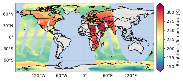
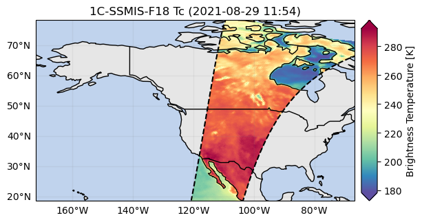
Now let’s plot this single PMW channel in the geographic space:
[ ]:
da.gpm.plot_map(add_swath_lines=False)
<cartopy.mpl.geocollection.GeoQuadMesh at 0x7f0abd9a6010>
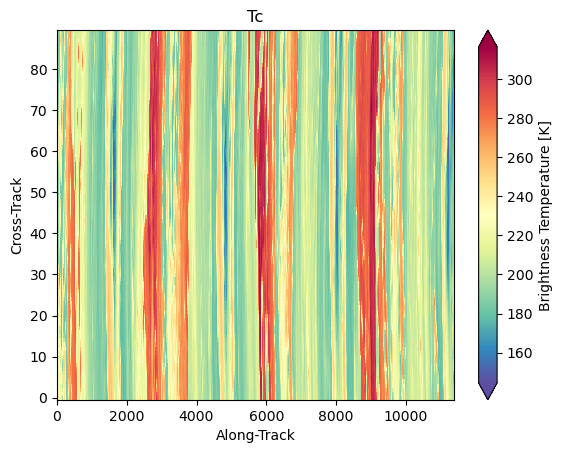
and now as an image, in “swath” view:
[ ]:
da.gpm.plot_image()
<matplotlib.image.AxesImage at 0x7f0abd5a6190>
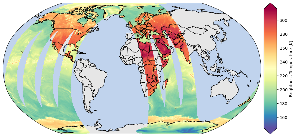
You can customize the map projection by passing a cartopy.crs.Projection to the subplot. The available projections are listed here.
[ ]:
# Define some figure options
dpi = 100
figsize = (12, 10)

# Example of Cartopy projections
crs_proj = ccrs.Robinson()  # ccrs.Orthographic(180, -90)

# Create the map
fig, ax = plt.subplots(subplot_kw={"projection": crs_proj}, figsize=figsize, dpi=dpi)
da.gpm.plot_map(ax=ax, add_labels=False, add_background=True, add_gridlines=False, add_swath_lines=False)
ax.set_global()
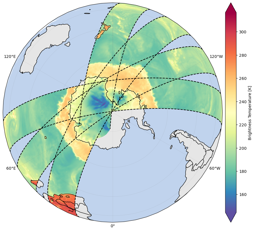
When working with PMW BT data, it’s often interesting also to have a look at the poles:
[ ]:
# Display South Pole
dpi = 100
figsize = (12, 10)
crs_proj = ccrs.Orthographic(180, -90)

fig, ax = plt.subplots(subplot_kw={"projection": crs_proj}, figsize=figsize, dpi=dpi)
with gpm.config.set({"viz_hide_antimeridian_data": False}):
    da.gpm.plot_map(ax=ax, add_swath_lines=True)
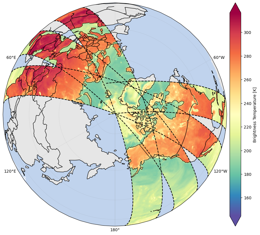
[ ]:
# Display North Pole
dpi = 100
figsize = (12, 10)
crs_proj = ccrs.Orthographic(180, 90)
fig, ax = plt.subplots(subplot_kw={"projection": crs_proj}, figsize=figsize, dpi=dpi)
with gpm.config.set({"viz_hide_antimeridian_data": False}):
    da.gpm.plot_map(ax=ax, add_swath_lines=True)
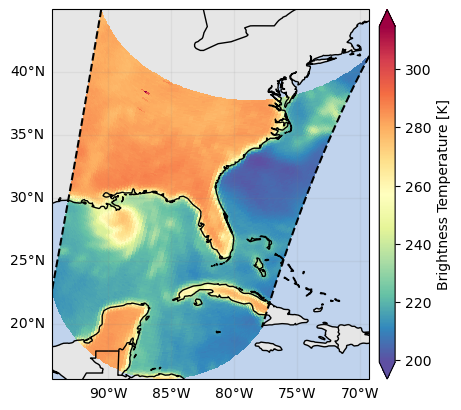
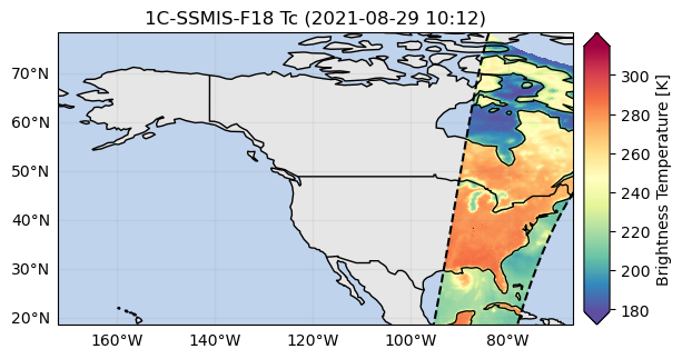
By focusing on a narrow region, it’s possible to better analyze fine-scale details and identify storms and precipitating clouds:
[ ]:
p = da.gpm.sel(gpm_id=slice(start_gpm_id, end_gpm_id)).gpm.plot_map()
p.axes.set_title(da.gpm.title(add_timestep=True))
Text(0.5, 1.0, '1C-SSMIS-F18 Tc (2021-08-29 13:00)')

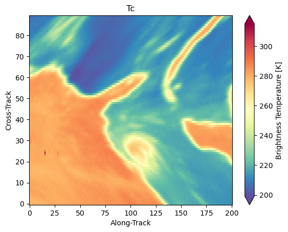
The same data, in swath view looks like this:
[ ]:
da.gpm.sel(gpm_id=slice(start_gpm_id, end_gpm_id)).gpm.plot_image()
<matplotlib.image.AxesImage at 0x7f0aac6ad590>
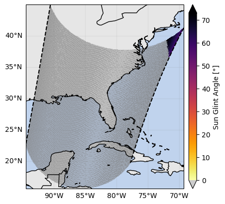
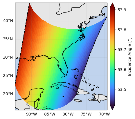
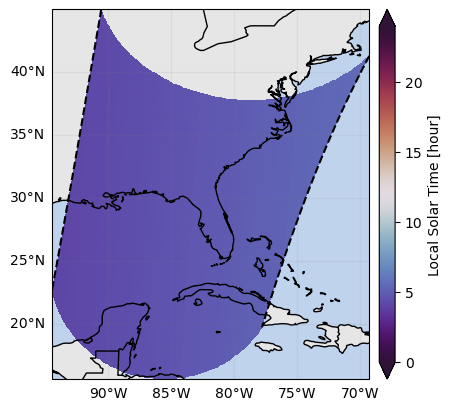
When we visualize different product variables, GPM-API will automatically try to use different appropriate colormaps and colorbars. You can observe this in the following example:
[ ]:
ds_subset = ds.gpm.sel(gpm_id=slice(start_gpm_id, end_gpm_id), pmw_frequency="19V", scan_mode="S1")
ds_subset["Tc"].gpm.plot_map()
ds_subset["sunGlintAngle"].gpm.plot_map()
ds_subset["incidenceAngle"].gpm.plot_map()
ds_subset["sunLocalTime"].gpm.plot_map()
<cartopy.mpl.geocollection.GeoQuadMesh at 0x7f0abcf39410>
GPM-API also provides FacetGrid capabilities, which allow you to plot multiple PMW channels in a single figure.
Now let’s first create a FacetGrid figure on a small region:
[ ]:
da_subset = ds.gpm.sel(gpm_id=slice(start_gpm_id, end_gpm_id))["Tc"]
fc = da_subset.gpm.plot_map(col="pmw_frequency", col_wrap=4)
fc.remove_title_dimension_prefix()
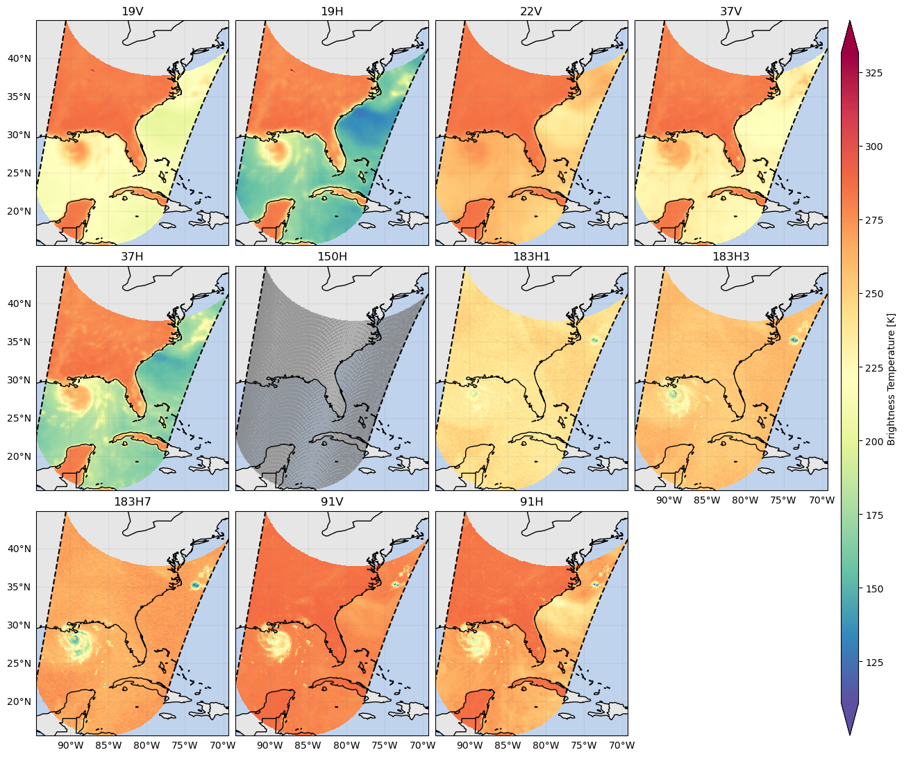
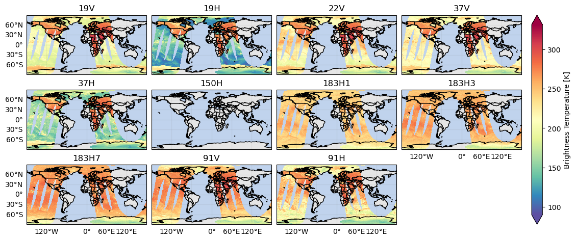
and now displaying the data acquired over multiple orbits:
[ ]:
fc = ds["Tc"].gpm.plot_map(col="pmw_frequency", col_wrap=4, add_swath_lines=False)
fc.remove_title_dimension_prefix()
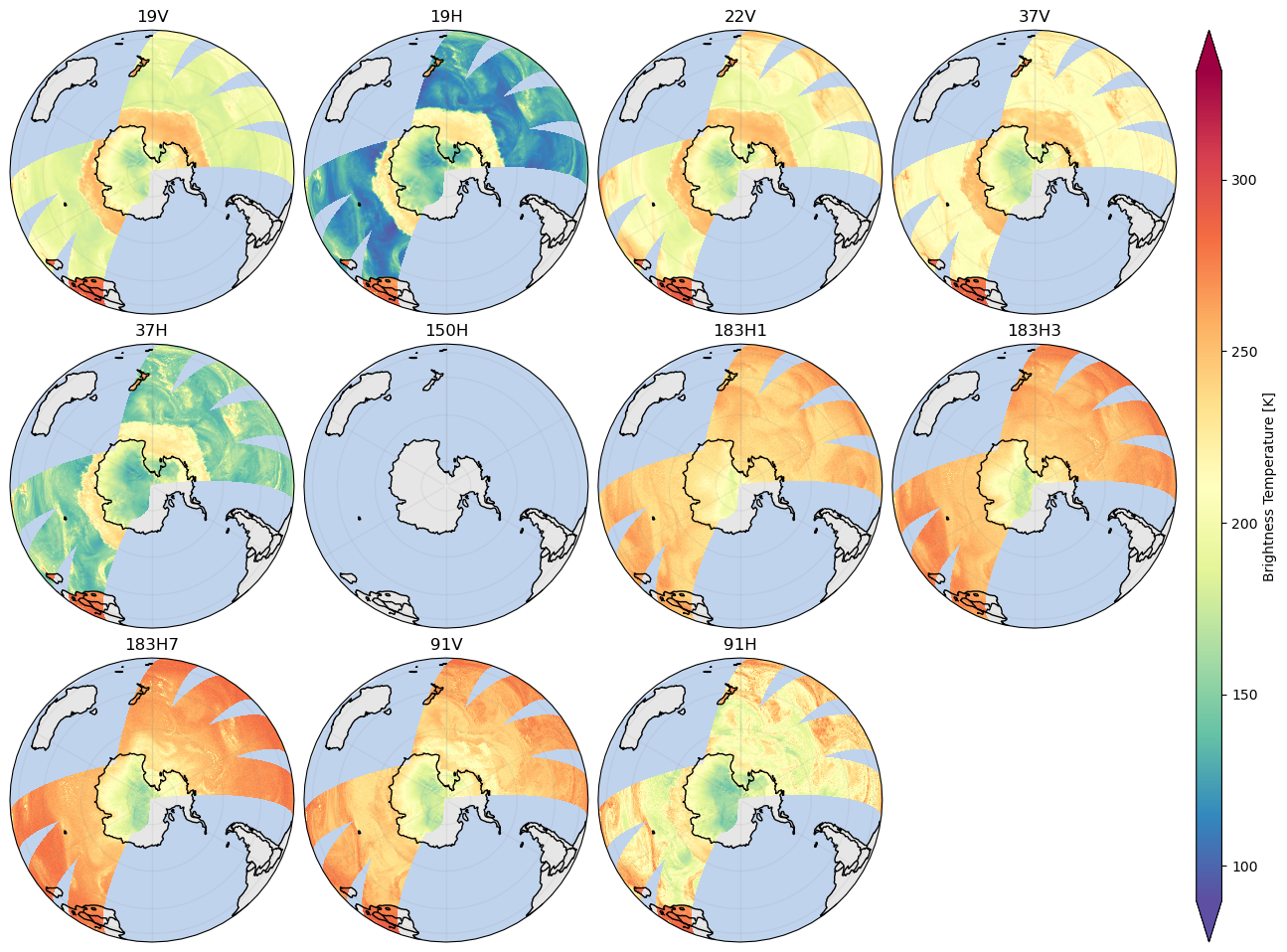
And now, just for fun, over the poles:
[ ]:
crs_proj = ccrs.Orthographic(180, -90)
with gpm.config.set({"viz_hide_antimeridian_data": False}):
    fc = ds["Tc"].gpm.plot_map(
        col="pmw_frequency",
        subplot_kwargs={"projection": crs_proj},
        col_wrap=4,
        add_swath_lines=False,
        add_labels=False,
    )
    fc.remove_title_dimension_prefix()
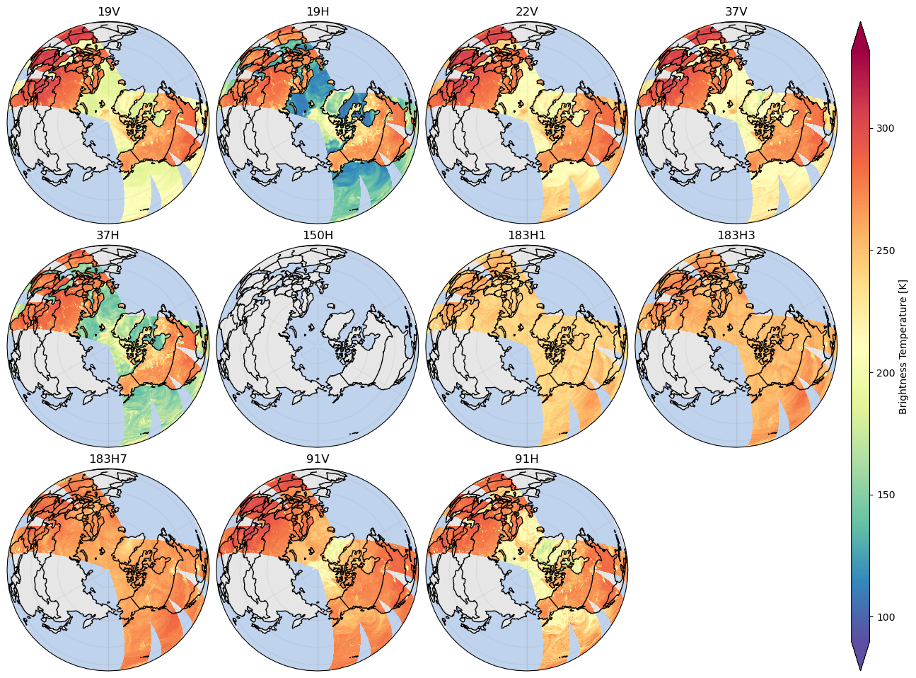
[ ]:
crs_proj = ccrs.Orthographic(180, 90)
with gpm.config.set({"viz_hide_antimeridian_data": False}):
    fc = ds["Tc"].gpm.plot_map(
        col="pmw_frequency",
        subplot_kwargs={"projection": crs_proj},
        col_wrap=4,
        add_swath_lines=False,
        add_labels=False,
    )
    fc.remove_title_dimension_prefix()
6. Community-based Retrievals#
GPM-API aims to be a platform where scientist can share their algorithms and retrievals with the community.
Based on the GPM product you are working with, you will have a series of retrievals available to you. For example, GPM-API currently provides the following retrievals for the 1C-PMW products:
[ ]:
ds.gpm.available_retrievals()
['PCA_RGB',
 'PCT',
 'PD',
 'PESCA',
 'PR',
 'UMAP_RGB',
 'polarization_corrected_temperature',
 'polarization_difference',
 'polarization_ratio',
 'rgb_composites']
The gpm.retrieve method enables to apply specific retrievals to your dataset.
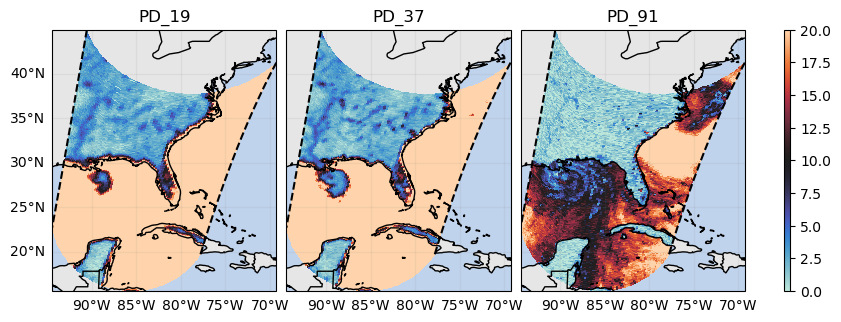
For example, it is possible to easily retrieve Polarization Difference (PD),Polarization Ratio (PR) and Polarization Corrected Temperature (PCT):
[ ]:
# Compute polarization difference
ds_pd = ds.gpm.retrieve("polarization_difference")  # ds.gpm.retrieve("PD")

# Compute polarization ratio
ds_pr = ds.gpm.retrieve("polarization_ratio")  # ds.gpm.retrieve("PR")

# Compute polarization correct temperature
# - Remove surface water signature on land brightness temperature
ds_pct = ds.gpm.retrieve("polarization_corrected_temperature")  # ds.gpm.retrieve("PCT")
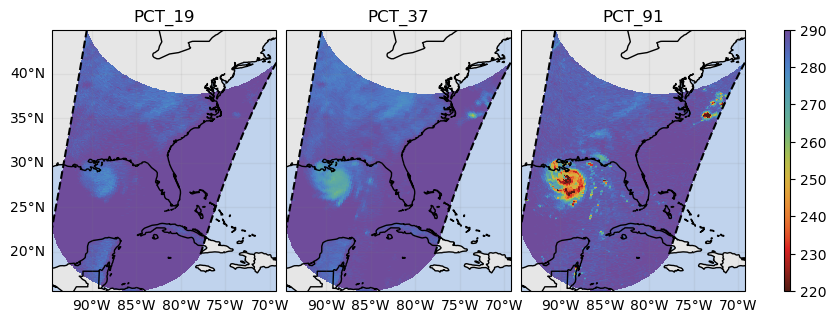
These PMW features can be easily visualized exploiting the GPM-API FacetGrid capabilities:
[ ]:
da_subset = ds_pct.gpm.sel(gpm_id=slice(start_gpm_id, end_gpm_id)).to_array("PCT")
fc = da_subset.gpm.plot_map(col="PCT", col_wrap=4, vmin=220, vmax=290, cmap="rainbow_PuBr_r")
fc.remove_title_dimension_prefix()
[ ]:
da_subset = ds_pd.gpm.sel(gpm_id=slice(start_gpm_id, end_gpm_id)).to_array("PD")
fc = da_subset.gpm.plot_map(col="PD", col_wrap=4, vmin=0, vmax=20, cmap="icefire")
fc.remove_title_dimension_prefix()
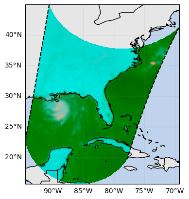
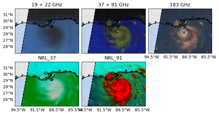
To facilitate the interpretation of the scenes, GPM-API also enable to generate a set of RGB composites on-the-fly.
[ ]:
# Retrieve RGB composites
ds_rgb = ds.gpm.retrieve("rgb_composites")
ds_rgb
<xarray.Dataset> Size: 83MB
Dimensions:             (along_track: 11377, cross_track: 90, rgb: 3)
Coordinates:
    SCorientation       (along_track) float32 46kB 0.0 0.0 0.0 ... 0.0 0.0 0.0
    lon                 (cross_track, along_track) float32 4MB 87.31 ... 9.236
    lat                 (cross_track, along_track) float32 4MB 86.83 ... -81.26
    time                (along_track) datetime64[ns] 91kB 2021-08-29T10:00:00...
    gpm_id              (along_track) <U10 455kB '61187-1561' ... '61191-51'
    gpm_granule_id      (along_track) int64 91kB 61187 61187 ... 61191 61191
    gpm_cross_track_id  (cross_track) int64 720B 0 1 2 3 4 5 ... 85 86 87 88 89
    gpm_along_track_id  (along_track) int64 91kB 1561 1562 1563 ... 49 50 51
    pmw_frequency       <U5 20B '22V'
    crsWGS84            int64 8B 0
  * rgb                 (rgb) <U1 12B 'r' 'g' 'b'
Dimensions without coordinates: along_track, cross_track
Data variables:
    19 + 22 GHz         (rgb, cross_track, along_track) float32 12MB 0.3615 ....
    37 + 91 GHz         (rgb, cross_track, along_track) float32 12MB 0.3236 ....
    183 GHz             (rgb, cross_track, along_track) float64 25MB 0.1911 ....
    NRL_37              (rgb, cross_track, along_track) float32 12MB 1.0 ... 0.0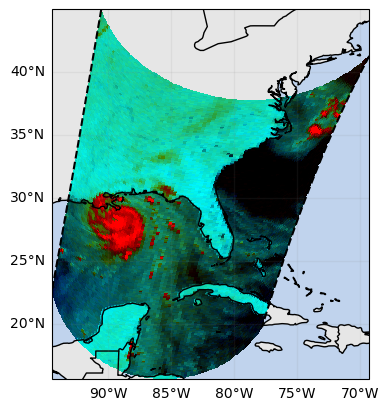
NRL_91 (rgb, cross_track, along_track) float32 12MB 0.9936 ....The Naval Research Laboratory (NRL) 37 and 89 GHz composites are commonly used to analyze the structure of tropical cyclones:
[ ]:
ds_rgb_subset = ds_rgb.gpm.sel(gpm_id=slice(start_gpm_id, end_gpm_id))
ds_rgb_subset["NRL_37"].gpm.plot_map(rgb="rgb")
ds_rgb_subset["NRL_91"].gpm.plot_map(rgb="rgb")
<cartopy.mpl.geocollection.GeoQuadMesh at 0x7f0aa0341c90>
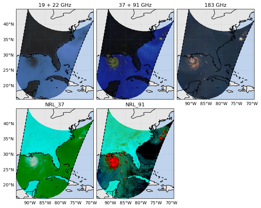
Again, all RGB composites can be displayed in a single figure using the FacetGrid capabilities.
[ ]:
ds_rgb_subset = ds_rgb.gpm.sel(gpm_id=slice(start_gpm_id, end_gpm_id))
fc = ds_rgb_subset.to_array(dim="composite").gpm.plot_map(col="composite", col_wrap=3, rgb="rgb")
fc.remove_title_dimension_prefix()
plt.show()
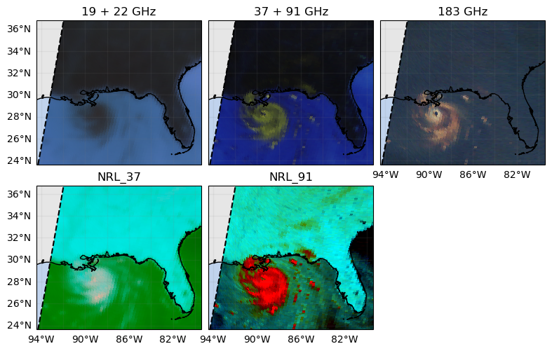
If you want to restrict the geographic extent of each figure panel around a particular area of interest, you can use the axis method set_extent.
Please be aware that rendering the figure with this approach can be quite slow, because plot_map plots first all the data, and then restrict the figure extent over the area of interest.
For more efficient scene cropping, see section 7.
[ ]:
extent = [-95, -85, 25, 32]
ds_rgb_subset = ds_rgb.gpm.sel(gpm_id=slice(start_gpm_id, end_gpm_id))
fc = ds_rgb_subset.to_array(dim="composite").gpm.plot_map(col="composite", col_wrap=3, rgb="rgb", optimize_layout=False)
fc.remove_title_dimension_prefix()
fc.set_extent(extent)
plt.show()
If you are analyzing a specific region, the gpm accessor method extent might be quite useful to zoom in/out:
[ ]:
ds_rgb_subset = ds_rgb.gpm.sel(gpm_id=slice(start_gpm_id, end_gpm_id))
# extent = ds_rgb_subset.gpm.extent(size=(10))  # set an extent of size 10 degrees around the scene center
extent = ds_rgb_subset.gpm.extent(
    padding=(0, -10, -8, -8),
)  # shrink the extent by 8 degrees in the North/South direction
fc = ds_rgb_subset.to_array(dim="composite").gpm.plot_map(col="composite", col_wrap=3, rgb="rgb", optimize_layout=False)
fc.remove_title_dimension_prefix()
fc.set_extent(extent)
plt.show()
7. Geospatial Manipulations#
GPM-API provides methods to easily spatially subset orbits by extent, country or continent.
Note however, that an area can be crossed by multiple orbits depending on the size of your GPM satellite dataset. In other words, multiple orbit slices in along-track direction can intersect the area of interest.
The method get_crop_slices_by_extent, get_crop_slices_by_country and get_crop_slices_by_continent enable to retrieve the orbit portions intersecting the area of interest.
[ ]:
# Subset the data for fast rendering and select single channel
da = ds["Tc"].isel(pmw_frequency=0)
# Crop by country
list_isel_dict = da.gpm.get_crop_slices_by_country("United States")
print(list_isel_dict)
# Crop by extent
extent = get_country_extent("United States")
list_isel_dict = da.gpm.get_crop_slices_by_extent(extent)
print(list_isel_dict)
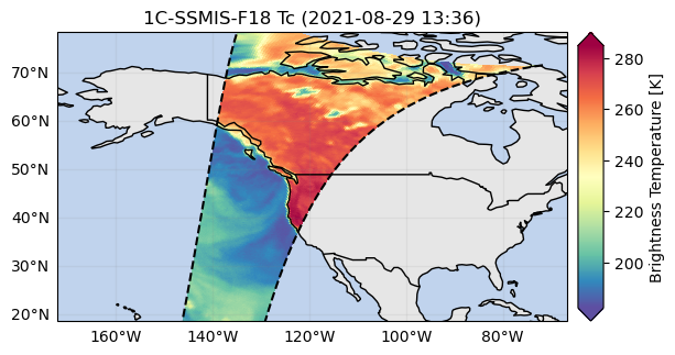
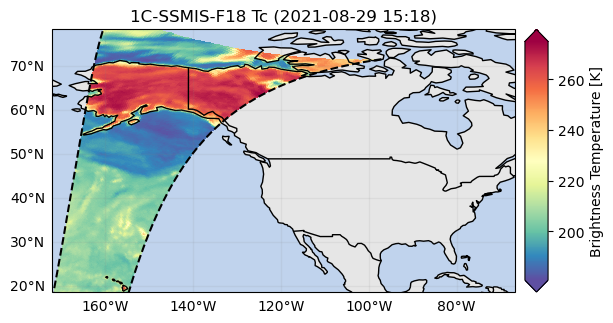
# Plot the swaths crossing the country
for isel_dict in list_isel_dict:
da_subset = da.isel(isel_dict)
slice_title = da_subset.gpm.title(add_timestep=True)
p = da_subset.gpm.plot_map()
p.axes.set_extent(extent)
p.axes.set_title(label=slice_title)
[{'along_track': slice(136, 675, None)}, {'along_track': slice(3327, 3896, None)}, {'along_track': slice(6540, 7118, None)}, {'along_track': slice(9761, 10339, None)}]
[{'along_track': slice(136, 675, None)}, {'along_track': slice(3327, 3896, None)}, {'along_track': slice(6540, 7118, None)}, {'along_track': slice(9761, 10339, None)}]
[ ]:
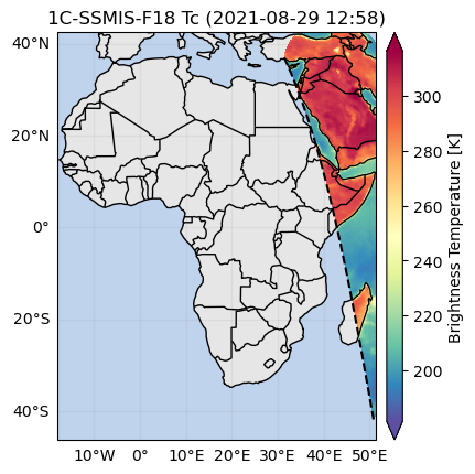
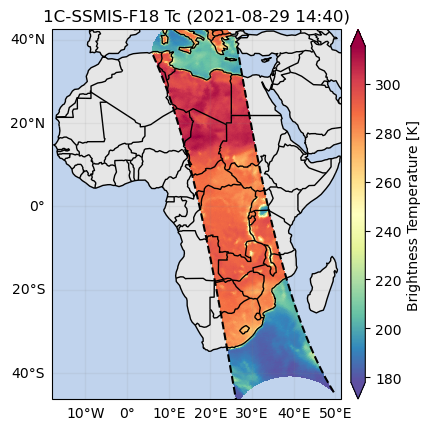
# Crop by continent
extent = get_continent_extent("Africa")
list_isel_dict = da.gpm.get_crop_slices_by_extent(extent)
list_isel_dict = da.gpm.get_crop_slices_by_continent("Africa")
print(list_isel_dict)

# - Plot the swath crossing the country
for isel_dict in list_isel_dict:
    da_subset = da.isel(isel_dict)
    slice_title = da_subset.gpm.title(add_timestep=True)
    p = da_subset.gpm.plot_map()
    p.axes.set_extent(extent)
    p.axes.set_title(label=slice_title)
[{'along_track': slice(5294, 6015, None)}, {'along_track': slice(8461, 9237, None)}]
You can also easily obtain the extent around a given point using the get_geographic_extent_around_point function and use the gpm accessor methods get_crop_slices_around_point or crop_around_point to subset your dataset:
[ ]:
# Crop around a point
lon = 32 # here near Lake Victoria in Africa
lat = 0.5
distance = 300_000 # 300 km
extent = get_geographic_extent_around_point(lon=lon, lat=lat, distance=distance)
list_isel_dict = da.gpm.get_crop_slices_by_extent(extent)
list_isel_dict = da.gpm.get_crop_slices_around_point(
lon=lon,
lat=lat,
distance=distance,
)
print(list_isel_dict)
# Define ROI coordinates
circle_lons, circle_lats = get_circle_coordinates_around_point(
lon,
lat,
radius=distance,
num_vertices=360,
)
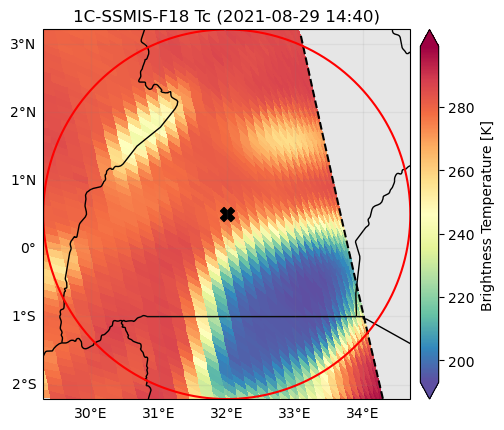
# Plot the swaths crossing the ROI
for isel_dict in list_isel_dict:
da_subset = da.isel(isel_dict)
slice_title = da_subset.gpm.title(add_timestep=True)
p = da_subset.gpm.plot_map()
p.axes.set_title(slice_title)
p.axes.plot(circle_lons, circle_lats, "r-", transform=ccrs.Geodetic())
p.axes.scatter(lon, lat, c="black", marker="X", s=100, transform=ccrs.Geodetic())
p.axes.set_extent(extent)
[{'along_track': slice(8815, 8906, None)}]
8. Feature Labelling#
Using the xarray ximage accessor, it is possible to delineate (label) specific features in the brightness temperature fields. The label array is added to the xarray object as a new coordinate.
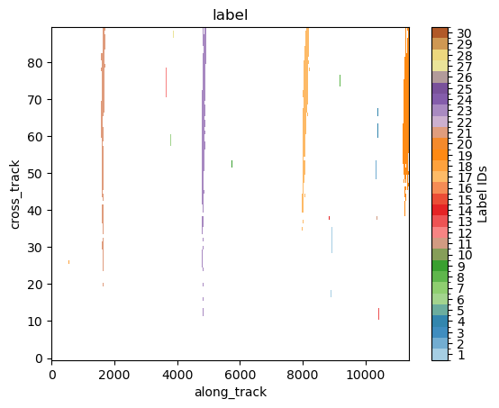
As an example, here below we select a 183 GHZ channel and we labels regions where the brightness temperature is below a certain threshold. These regions will likely correspond to precipitating areas.
[ ]:
da = ds["Tc"].sel(pmw_frequency="183H7")
[ ]:
# Retrieve labeled xarray object
label_name = "label"
da = da.ximage.label(
    max_value_threshold=175,  # K
    min_area_threshold=5,
    footprint=5,  # assign same label to precipitating areas 5 pixels apart
    sort_by="minimum",  # "area", "maximum", "minimum", <custom_function>
    sort_decreasing=False,
    label_name=label_name,
)
# Plot full label array
da[label_name].ximage.plot_labels()
<matplotlib.image.AxesImage at 0x7fd4306c4590>
9. Patch Extraction#
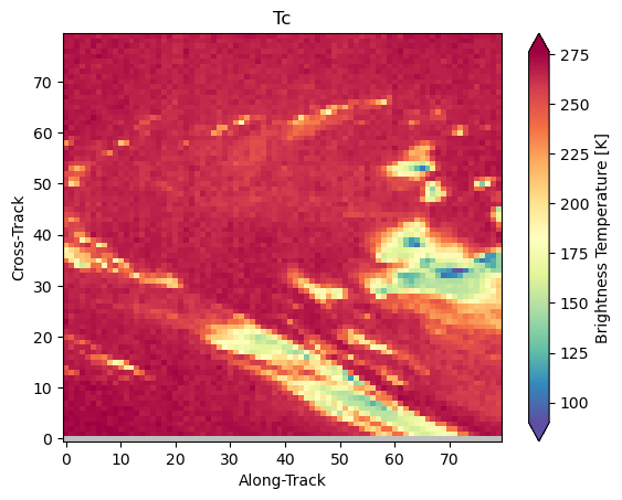
With the xarray ximage accessor, it is also possible to extract patches around labels. Here we provide a minimal example on how to proceed:
[ ]:
# Define the patch generator
da_patch_gen = da.ximage.label_patches(
    label_name=label_name,
    patch_size=(80, 80),
    # Output options
    n_patches=25,
    # Patch extraction Options
    padding=0,
    centered_on="max",
    # Tiling/Sliding Options
    debug=False,
    verbose=False,
)

# # Retrieve list of patches
list_label_patches = list(da_patch_gen)
list_da = [da for label, da in list_label_patches]

# Display two patches
gpm.plot_patches(list_label_patches[:2])
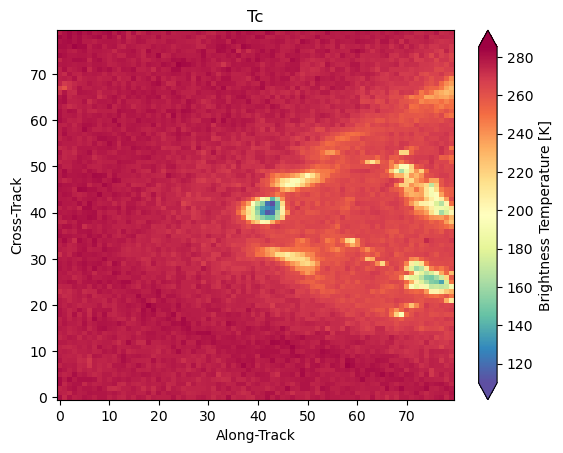
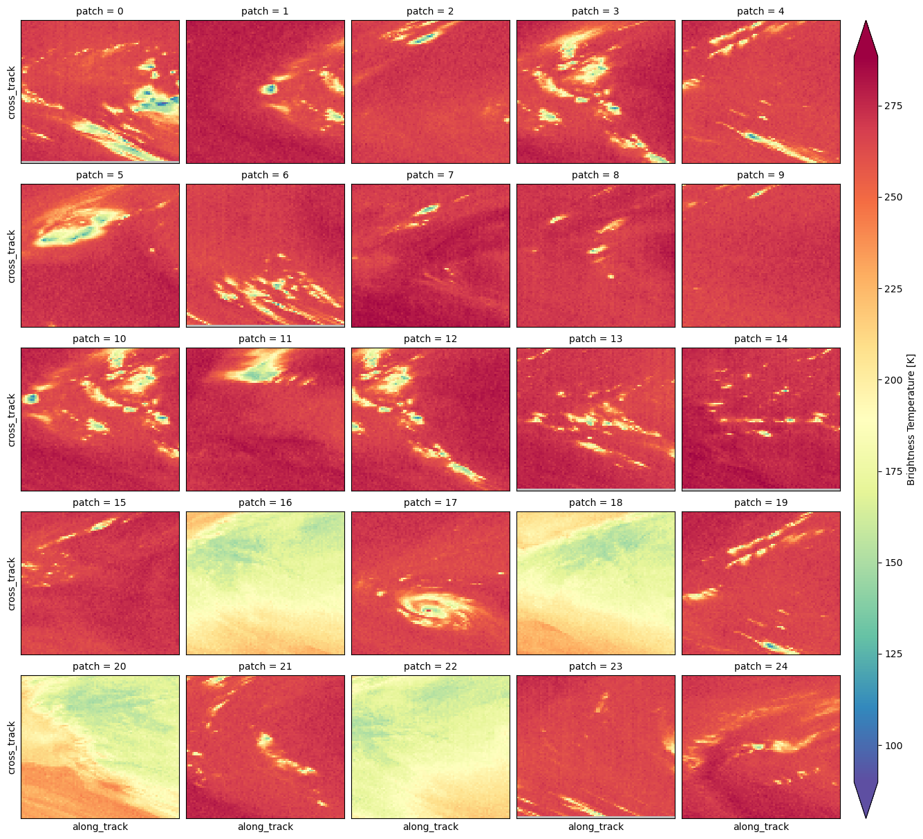
You can once again exploit the xarray manipulations and FacetGrid capabilities to quickly create the following figure:
[ ]:
list_da_without_coords = [da.drop_vars(["lon", "lat"]) for da in list_da]
da_patch = xr.concat(list_da_without_coords, dim="patch")
da_patch.isel(patch=slice(0, 25)).gpm.plot_image(col="patch", col_wrap=5)
<gpm.visualization.facetgrid.ImageFacetGrid at 0x7fd40c1c0950>